50 results for materials science

Partitioning the vibrational spectrum: Fingerprinting defects in solids

Graphical abstract Computational Materials Science 181, 109736 (2020)
Authors:  Danny E. P. Vanpoucke
Journal: Computational Materials Science 181, 109736 (2020)
doi: 10.1016/j.commatsci.2020.109736
IF(2019): 2.863
export: bibtex
pdf: <ComputMaterSci>   (Open Access)
github: <Hive-toolbox>


Graphical abstract Computational Materials Science 181, 109736 (2020)
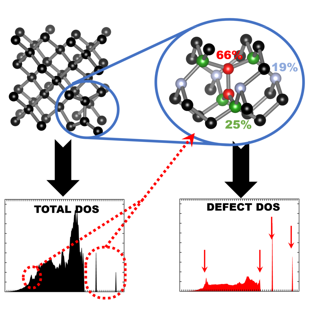
Graphical Abstract: Finger printing defects in diamond through the creation of the vibrational spectrum of a defect.

Abstract

Vibrational spectroscopy techniques are some of the most-used tools for materials
characterization. Their simulation is therefore of significant interest, but commonly
performed using low cost approximate computational methods, such as force-fields.
Highly accurate quantum-mechanical methods, on the other hand are generally only used
in the context of molecules or small unit cell solids. For extended solid systems,
such as defects, the computational cost of plane wave based quantum mechanical simulations
remains prohibitive for routine calculations. In this work, we present a computational scheme
for isolating the vibrational spectrum of a defect in a solid. By quantifying the defect character
of the atom-projected vibrational spectra, the contributing atoms are identified and the strength
of their contribution determined. This method could be used to systematically improve phonon
fragment calculations. More interestingly, using the atom-projected vibrational spectra of the
defect atoms directly, it is possible to obtain a well-converged defect spectrum at lower
computational cost, which also incorporates the host-lattice interactions. Using diamond as
the host material, four point-defect test cases, each presenting a distinctly different
vibrational behaviour, are considered: a heavy substitutional dopant (Eu), two intrinsic
point-defects (neutral vacancy and split interstitial), and the negatively charged N-vacancy
center. The heavy dopant and split interstitial present localized modes at low and high
frequencies, respectively, showing little overlap with the host spectrum. In contrast, the
neutral vacancy and the N-vacancy center show a broad contribution to the upper spectral range
of the host spectrum, making them challenging to extract. Independent of the vibrational behaviour,
the main atoms contributing to the defect spectrum can be clearly identified. Recombination of
their atom-projected spectra results in the isolated spectrum of the point-defect.

New year’s resolution

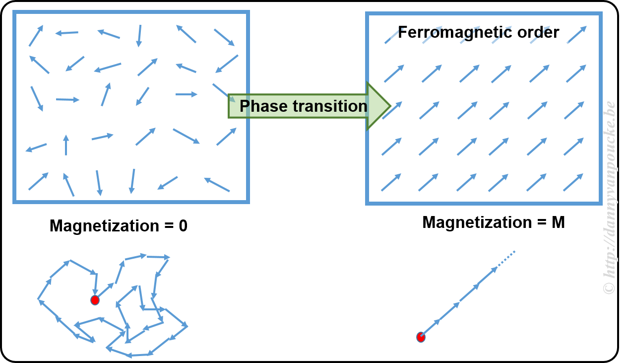
A new year, a new beginning.
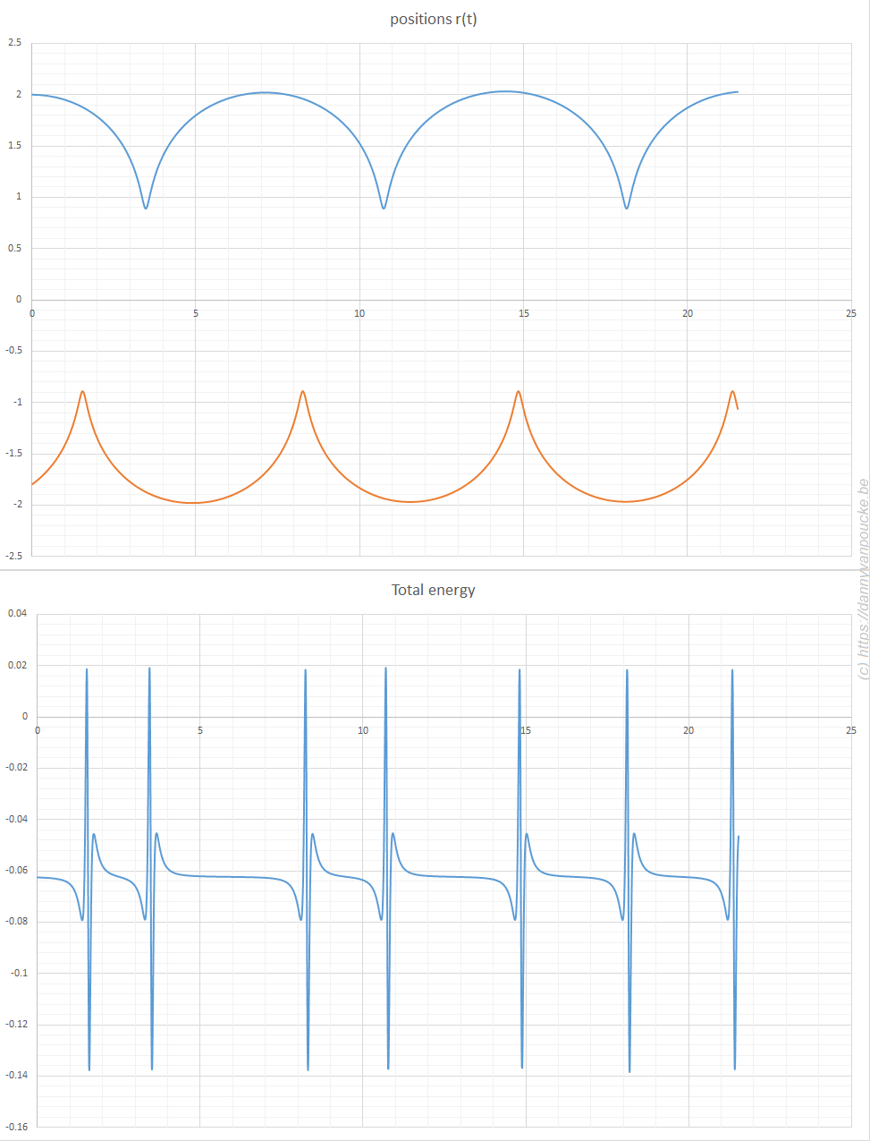
For most people this is a time of making promises, starting new habits or stopping old ones. In general, I forgo making such promises, as I know they turn out idle in a mere few weeks without external stimulus or any real driving force.

In spite of this, I do have a new years resolution for this year: I am going to study machine learning and use it for any suitable application I can get my hands on (which will mainly be materials science, but one never knows).  I already have a few projects in mind, which should help me stay focused and on track. With some luck, you will be reading about them here on this blog. With some more luck, they may even end up being part of an actual scientific publication.

But first things first, learn the basics (beyond hear-say messages of how excellent and world improving AI is/will be). What are the different types of machine learning available, is it all black box or do you actually have some control over things. Is it a kind of magic? What’s up with all these frameworks (isn’t there anyone left who can program?), and why the devil seem they all to be written in a script langue (python) instead of a proper programming language? A lot of questions I hope to see answered. A lot of things to learn. Lets start by building some foundations…the old fashioned way: By studying using a book, with real paper pages!

Happy New Year, and best wishes to you all!

Building bridges towards experiments.

Finding a minimum using Metropolis Monte Carlo.

Quantum Holy Grail: The Ground-State

Quantum mechanical calculations provide a powerful tool to investigate the world around us. Unfortunately it is also a computationally very expensive tool to use, which puts a boundary on what is possible in terms of computational materials research. For example, when investigating a solid at the quantum mechanical level, you are limited in the number of atoms that you can consider. Even with a powerful supercomputer at hand, a hundred to a thousand atoms are currently accessible for “routine” investigations. The computational cost also limits the number of configurations/combinations you can calculate.

However, in the end— and often with some blood sweat and tears—these calculations do provide you the ground-state structure and energy of your system. From this point forward you can continue characterizing its properties, life is beautiful and happy times are just beyond the horizon. At this horizon your experimental colleague awaits you. And he/she tells you:

Sorry, I don’t find that structure in my sample.

After recovering from the initial shock, you soon realize that in (materials science) experiments one seldom encounters a sample in “the ground-state”. Experiments are performed at temperatures above 0K and pressures above 0 Pa (even in vacuum :p ). Furthermore, synthesis methods often involve elevated temperatures, increased pressure, mechanical forces, chemical reactions,… which give rise to meta-stable configurations. In such an environment, your nicely deduced ground-state may be an exception to the rule. It is only one point within the phase-space of the possible.

So how can you deal with this? You somehow need to sample the phase-space available to the experiment.

Sampling Phase-Space for Ball-milling synthesis.

For a few years now, I have a very fruitful collaboration with Prof. Rounaghi. His interest goes toward the cheap fabrication of metal-nitrides. Our first collaboration focused on AlN, while later work included Ti, V and Cr-nitrides. Although this initial work had a strong focus on simple corroboration through the energies calculated at the quantum mechanical level, the collaboration also allowed me to look at my data in a different way. I wanted to “simulate” the reactions of ball-milling experiments more closely.

Due to the size-limitations of quantum mechanical calculations I played with the following idea:

  • Assume there exists a general master reaction which describes what happens during ball-milling.

X Al + Y Melamine → x1 Al + x2 Melamine + x3 AlN + …

where all the xi represent the fractions of the reaction products present.

  • With the boundary condition that the number of particles needs to be conserved, you end up with a large set of (x1,x2,x3,…) configurations which each have a certain energy. This energy is calculated using the quantum mechanical energies of each product. The configuration with the lowest energy is the ground state configuration. However, investigating the entire accessible phase-space showed that the energies of the other possible configurations are generally not that much higher.
  • What if we used the energy available due to ball-milling in the same fashion as we use kBT? And sample the phase-space using Boltzmann statistics.
  • The resulting Boltzmann distribution of the configurations available in the phase-space can then be used to calculate the mass/atomic fraction of each of the products and allow us to represent an experimental sample as a collection of small units with slightly different configurations, weighted according to their Boltzmann distribution.

This setup allowed me to see the evolution in end-products as function of the initial ratio in case of AlN, and in our current project to indicate the preferred Iron-nitride present.

Grid-sampling vs Monte-Carlo-sampling

Whereas the AlN system was relatively easy to investigate—the phase space was only 3 dimensional— the recent iron based system ended up being 4 dimensional when considering only host materials, and 10 dimensional when including defects. For a small 3-4D phase-space, it is possible to create an equally spaced grid and get converged results using a few million to a billion grid-points. For a 10D phase-space this is no longer possible. As you can no longer keep all data-points (easily) in storage during your calculation (imagine 1 Billion points, requiring you to store 11 double precision floats or about 82Gb) you need a method that does not rely on large arrays of data. For our Boltzmann statistics this gives us a bit of a pickle, as we need to have the global minimum of our phase space. A grid is too course to find it, while a simple Monte-Carlo just keeps hopping around.

Using Metropolis’s improvement of the Monte-Carlo approach was an interesting exercise, as it clearly shows the beauty and simplicity of the approach. This becomes even more awesome the moment you imagine the resources available in those days. I noted 82Gb being a lot, but I do have access to machines with those resources; its just not available on my laptop. In those days MANIAC supercomputers had less than 100 kilobyte of memory.

Although I theoretically no longer need the minimum energy configuration, having access to that information is rather useful. Therefore, I first search the phase-space for this minimum. This is rather tricky using Metropolis Monte Carlo (of course better techniques exist, but I wanted to be a bit lazy), and I found that in the limit of T→0 the algorithm will move toward the minimum. This, however, may require nearly 100 million steps of which >99.9% are rejected. As it only takes about 20 second on a modern laptop…this isn’t a big issue.

Finding a minimum using Metropolis Monte Carlo.

Finding a minimum using Metropolis Monte Carlo.

Next, a similar Metropolis Monte Carlo algorithm can be used to sample the entire phase space. Using 109 sample points was already sufficient to have a nicely converged sampling of the phase space for the problem at hand. Running the calculation for 20 different “ball-milling” energies took less than 2 hours, which is insignificant, when compared to the resources required to calculate the quantum mechanical ground state energies (several years). The figure below shows the distribution of the mass fraction of one of the reaction products as well as the distribution of the energies of the sampled configurations.

Metropolis Monte Carlo distribution of mass fraction and configuration energies for 3 sets of sample points.

Metropolis Monte Carlo distribution of mass fraction and configuration energies for 3 sets of sample points.

This clearly shows us how unique and small the quantum mechanical ground state configuration and its contribution is compared to the remainder of the phase space. So of course the ground state is not found in the experimental sample but that doesn’t mean the calculations are wrong either. Both are right, they just look at reality from a different perspective. The gap between the two can luckily be bridged, if one looks at both sides of the story. 


Functional Molecular Modelling: simulating particles in excel

Molecular dynamics in excel. A system of three particles on a line, with one particle fixed at 0. All particles interact through a Lennard-Jones potential. The Molecular dynamics simulation shows how the particles move as time evolves. Their positions are updated using the leap-frog algorithm. The extreme hard nature of the Lennard-Jones potential gives rise to the sharp spikes in the total energy. It is this last aspect which causes the straight forward implementation of Newton's equations of motion to fail.

This semester I had several teaching assignments. I was a TA for the course biophysics for the first bachelor biomedical sciences, supervised two 3rd bachelor students physics during their first steps in the realm of computational materials science, and finally, I was responsible for half the course Functional Molecular Modelling for the first Masters Biomedical students (Bioelectronics and Nanotechnology). In this course, I introduce the the students into the basic concepts of classical molecular modelling (quantum modelling is covered by Prof. Wilfried Langenaeker). It starts with a reiteration of some basic concepts from statistics and moves on to cover the canonical ensemble. Things get more interesting with the introduction into Monte-Carlo(MC) and Molecular Dynamics(MD), where I hope to teach the students the basics needed to perform their own MC and MD simulations. This also touches the heart of what this course should cover. If I hear a title like Functional Molecular Modelling, my thoughts move directly to practical applications, developing and implementing models, and performing simulations. This becomes a bit difficult as none of the students have any programming experience or skills.

Luckily there is excel. As the basic algorithms for MC and MD are actually quite simple, this office package can be (ab)used to allow the students to perform very simple simulations. This even without the use of macro’s or any advanced features. Because Excel can also plot the data present in the cells, you immediately see how properties of the simulated system vary during the simulation, and you get direct update of all graphs every time a simulation is run.

It seems I am not the only one who is using excel for MD simulations. In 1995, Fraser and Woodcock even published a paper detailing the use of excel for performing MD simulations on a system of 100 particles. Their MD is a bit more advanced than the setup I used as it made heavy use of macro’s and needed some features to speed things up as much as possible. With the x486 66MHz computers available at that time, the simulations took of the order of hours. Which was impressive, as they served as an example of how computational speed had improved over the years, and compared to the months of supercomputer resources one of the authors had needed 25 years earlier to perform the same thing for his PhD. Nowadays the same excel simulation should only take minutes, while an actual program in Fortran or C may even execute the same thing in a matter of seconds or less.

For the classes and exercises, I made use of a simple 3-atom toy-model with Lennard-Jones interactions. The resulting simulations remain clear allowing their use for educational purposes. In case of  MC simulations, a nice added bonus is the fact that excel updates all its fields automatically when a cell is modified. As a result, all random numbers are regenerated and a new simulation can be performed by saving the excel-sheet or just modifying a not-used cell.

Monte Carlo in excel. A system of three particles on a line, with one particle fixed at 0. All particles interact through a Lennard-Jones potential. The Monte Carlo simulation shows how the particles move toward their equilibrium position.

Monte Carlo in excel. A system of three particles on a line, with one particle fixed at 0. All particles interact through a Lennard-Jones potential. The Monte Carlo simulation shows how the particles move toward their equilibrium position.

The simplicity of Newton’s equations of motion make it possible to perform simple MD simulations, and already for a three particle system, you can see how unstable the algorithm is. Implementation of the leap-frog algorithm isn’t much more complex and shows incredible the stability of this algorithm. In the plot of the total energy you can even see how the algorithm fights back to retain stability (the spikes may seem large, but the same setup with a straight forward implementation of Newton’s equation of motion quickly moves to energies of the order of 100).

Molecular dynamics in excel. A system of three particles on a line, with one particle fixed at 0. All particles interact through a Lennard-Jones potential. The Molecular dynamics simulation shows how the particles move as time evolves. Their positions are updated using the leap-frog algorithm. The extreme hard nature of the Lennard-Jones potential gives rise to the sharp spikes in the total energy. It is this last aspect which causes the straight forward implementation of Newton's equations of motion to fail.

Molecular dynamics in excel. A system of three particles on a line, with one particle fixed at 0. All particles interact through a Lennard-Jones potential. The Molecular dynamics simulation shows how the particles move as time evolves. Their positions are updated using the leap-frog algorithm. The extreme hard nature of the Lennard-Jones potential gives rise to the sharp spikes in the total energy. It is this last aspect which causes the straight forward implementation of Newton’s equations of motion to fail.


Review of 2016

2016 has come and gone. 2017 eagerly awaits getting acquainted. But first we look back one last time, trying to turn this into a tradition. What have I done during the last year of some academic merit.

Publications: +4

Completed refereeing tasks: +5

  • ACS Sustainable Chemistry & Engineering
  • The Journal of Physical Chemistry
  • Journal of Physics: Condensed Matter (2x)
  • Diamond and Related Materials

Conferences: +4 (Attended) & + 1 (Organized)

PhD-students: +2

  • Arthur De Vos : (Jan.-Mar., Ghent University, Ghent, Belgium )
  • Mohammadreza Hosseini (okt.-… ,Phd student physical chemistry, Tarbiat Modares University, Teheran, Iran)

Current size of HIVE:

  • 47K lines of program (code: 70 %)
  • 70 files
  • 44 (command line) options

Hive-STM program:

And now, upward and onward, a new year, a fresh start.

Bachelor projects @ UHasselt/IMO

Black arts of computational materials science.

Today the projects for the third year bachelor students in physics were presented at UHasselt. I also contributed two projects, giving the students the opportunity to choose for a computational materials science project. During these projects, I hope to introduce them into the modern (black) arts of High-Performance Computing and materials modelling beyond empirical models.

The two projects focus each on a different aspect of what it is to be a computational materials scientist. One project focuses on performing quantum mechanical calculations using the VASP program, and analyzing the obtained results with existing software. This student will investigate the NV-defect complex in diamond in all its facets. The other project focuses on the development of new tools to investigate the data generated by simulation software like VASP. This student will extend the existing phonon module in the HIVE-toolbox and use it to analyse a whole range of materials, varying from my favourite Metal-Organic Framework to a girl’s best friend: diamond.

Calculemus solidi


A description of the projects in Dutch can be found here.

MRS seminar: Topological Insulators

Bart Sorée receives a commemorative frame of the event. Foto courtesy of Rajesh Ramaneti.

Today I have the pleasure of chairing the last symposium of the year of the MRS chapter at UHasselt. During this invited lecture, Bart Sorée (Professor at UAntwerp and KULeuven, and alumnus of my own Alma Mater) will introduce us into the topic of topological insulators.

This topic became unexpectedly a hot topic as it is part of the 2016 Nobel Prize in Physics, awarded last Saturday.

This year’s Nobel prize in physics went to: David J. Thouless (1/2), F. Duncan M. Haldane (1/4) and J. Michael Kosterlitz (1/4) who received it

“for theoretical discoveries of topological phase transitions and topological phases of matter.”

On the Nobel Prize website you can find this document which gives some background on this work and explains what it is. Beware that the explanation is rather technical and at an abstract level. They start with introducing the concept of an order parameter. You may have heard of this in the context of dynamical systems (as I did) or in the context of phase transitions. In the latter context, order parameters are generally zero in one phase, and non-zero in the other. In overly simplified terms, one could say an order parameter is a kind of hidden variable (not to be mistaken for a hidden variable in QM) which becomes visible upon symmetry breaking. An example to explain this concept.

Example: Magnetization of a ferromagnet.

In a ferromagnetic material, the atoms have what is called a spin (imagine it as a small magnetic needle pointing in a specific direction, or a small arrow). At high temperature these spins point randomly in all possible directions, leading to a net zero magnetization (the sum of all the small arrows just lets you run in circles going nowhere). This magnetization is the order parameter. At the high temperature, as there is no preferred direction, the system is invariant under rotation and translations (i.e. if you shift it a bit or you rotate it, or both you will not see a difference) When the temperature is lower, you will cross what is called a critical temperature. Below this temperature all spins will start to align themselves parallel, giving rise to a non-zero magnetization (if all arrows point in the same direction, their sum is a long arrow in that direction). At this point, the system has lost the rotational invariance (because all spins point in  direction, you will know when someone rotated the system) and the symmetry is said to have broken.

Within the context of phase transitions, order parameters are often temperature dependent. In case of topological materials this is not the case. A topological material has a topological order, which means both phases are present at absolute zero (or the temperature you will never reach in any experiment no matter how hard you try) or maybe better without the presence of temperature (this is more the realm of computational materials science, calculations at 0 Kelvin actually mean without temperature as a parameter). So the order parameter in a topological material will not be temperature dependent.

Topological insulators

To complicate things, topological insulators are materials which have a topological order which is not as the one defined above 😯 —yup why would we make it easy 🙄 . It gets even worse, a topological insulator is conducting.

OK, before you run away or loose what is remaining of your sanity. A topological insulator is an insulating material which has surface states which are conducting. In this it is not that different from many other “normal” insulators. What makes it different, is that these surface states are, what is called, symmetry protected. What does this mean?

In a topological insulator with 2 conducting surface states, one will be linked to spin up and one will be linked to spin down (remember the ferromagnetism story of before, now the small arrows belong to the separate electrons and exist only in 2 types: pointing up=spin up, and pointing down=spin down). Each of these surface states will be populated with electrons. One state with electrons having spin up, the other with electrons having spin down. Next, you need to know that these states also have a real-space path let the electrons run around the edge of material. Imagine them as one-way streets for the electrons. Due to symmetry the two states are mirror images of one-another. As such, if electrons in the up-spin state more left, then the ones in the down-spin state move right. We are almost there, no worries there is a clue. Now, where in a normal insulator with surface states the electrons can scatter (bounce and make a U-turn) this is not possible in a topological insulator. But there are roads in two directions you say? Yes, but these are restricted. And up-spin electron cannot be in the down-spin lane and vice versa. As a result, a current going in such a surface state will show extremely little scattering, as it would need to change the spin of the electron as well as it’s spatial motion. This is why it is called symmetry protected.

If there are more states, things get more complicated. But for everyone’s sanity, we will leave it at this.  😎

Modern art in research.

Which combination to take?

Which combination to take?

Although it looks a bit like a modern piece of art, it is one more attempt at trying to find an optimum combination of parameters.

I’m currently trying to find “the best choice” for U and J for a DFT+U based project… DFT??? Density Functional Theory. This is an approximate method which is used in computational materials science to calculate the quantum mechanical behavior of electrons in matter. Instead of solving the Schrödinger equation, known from any quantum mechanic course, one solves the Hohenberg-Kohn-Sham equations. In these equations it are not the electrons which play a central role (which they do in the Schrödinger equations) but the electron density. Hohenberg, Kohn and Sham were able to show that their equations give the exact same results as the Schrödinger equations. There is, however, one small caveat: you need to have an “exact” exchange-correlation functional (a functional is just a function of a function). Unfortunately there is no known analytic form for this functional, so one needs to use approximated functionals. As you probably guessed, with these approximate functionals the solution of the Hohenberg-Kohn-Sham equations is no longer an exact solution.

For some molecules or solids the error is much larger than average due to the error in the exchange-correlation functional. These systems are therefore called “strongly-correlated” systems. Over the years, several ways have been devised to solve this problem in DFT. One of them is called DFT+U. It entails adding additional coulomb interactions (Hubbard-U-potential) between the “strongly interacting electrons”. However this additional interaction depends on the system at hand, so one always needs to fit this parameter against one of more properties one is interested in. The law of conservation of misery, however, makes sure that improving one property goes hand in hand with a deterioration of another property.

Since actual DFT+U has two independent parameters (U and J, though for many systems they can be dependent reducing to a single parameter) I had quite some fun running calculations for a 21×21 grid of possible pairs. Afterward, collecting the data I wanted to use for fitting purposes took my script about 2h! 😯 Unfortunately the 10 properties of interest I wanted to fit give optimum (U,J)-pair all over the grid. In the picture above, you see my most recent attempt at trying to deal with them. It shows for the entire grid how many of the 10 properties are reasonably well fit.There are two regions which fit 6 properties; One around (U,J)=(5,10) and another around (U,J)=(8.5,17.5). There will be more work before this gives a satisfactory result, the show will go on.

Annual Meeting of the Belgian Physical Society 2016

Belgian Physical Society Meeting 2016

ConferenceLogoWebsite_1

Wednesday May 18th was a good day for our little family. Since my girlfriend an I both are physicists by training, we attended the annual meeting of the Belgian Physical Society in Ghent, together. What made this event even more special was the fact that both of us had an oral presentation at the same conference, which never happened before. 🙂

Sylvia talked about an example of indeterminism in Newtonian mechanics, and showed how the indeterminism can be clarified by using non-standard analysis. The example considers the Norton Dome, a hill with a specifically designed shape ( y(x)=-2/3(1-(1-3/2|x|)^{2/3})^{3/2} ). When considering a point mass, experiencing only gravitational force, there are two solutions for the equation of motion: (1) the mass is there, and remains there forever (r(t)=0) and (2) the mass was rolling uphill with a non-zero speed which becomes exactly zero at the top, and continues over the top (  r(t)=\frac{1}{144} (t-T)^4 with T the time the top is reached). Here, r refers to the arc length as measured along the dome (0 at the top). In addition, there also exists a family of solutions taking the first solution at t<T, while taking the second solution at t>T. (As the first and second derivatives of these latter solutions are continuous, Newton will not complain.) This leads to indeterminism in a Newtonian system; for instance, you start with a mass on the top of the hill, and at a random point in time it starts to roll off without the presence of an external something putting it into motion. Using infinitesimals, Sylvia shows that the probability for the mass to start rolling off the dome immediately is infinitesimally close to one.

My own talk was on the use of computational materials science as a means for understanding and explaining experimental observations. I presented results on the pressure-induced breathing of the MIL-47(V) MOF, showing how the experimentally observed S-shape of the transition-pressure-curve can be explained by the spin interactions of the unpaired vanadium-d electrons: it turns out that regions with only ferromagnetic chains compress already at 85 MPa, while the addition of higher and higher percentages of anti-ferromagnetic chains increases the pressure at which the pores collapse, up to 125 MPa for the regions containing 100% anti-ferromagnetic chains. As a second topic, I showed how the electronic band structure of the linker-functionalized UiO-66(Zr) MOF changes. When one or two -OH or -SH groups are added to the benzene ring of the linker, part of the valence band is split off and moves into the band gap. In semiconductors, this would be called a gap state; however, in this case, since every linker in the material contributes

Belgian Physical Society Meeting 2016

Top left: I am presenting computational results on MOFs. Top Right: Sylvia presents the Norton Dome. Bottom: Group picture at the central garden in “Het Pand”. (Photos: courtesy of Sylvia Wenmackers (TL), Philippe Smet (TR), and Michael Tytgat (B) )

a single electron state to this gap state, it practically becomes the valence band top. As a consequence, the color of such functionalized MOF’s changes from white to yellow and orange. As a third topic, I discussed the COK-69(Ti) MOF. In this MOF the electrons in the titaniumoxide clusters are strongly correlated, just as for pure titaniumoxide. Because such systems are poorly described with standard DFT, we used the DFT+U approach, which allowed us to discern between Ti3+ and Ti4+ ions. The latter was practically done by partitioning the electron density using the Hirshfeld-I scheme.

Next to our own talks, the BPS-meeting started with two very interesting plenary lectures on the two big machines/facilities of the physics community: ITER (fusion reactor under construction) and LHC (circular collider, under constant upgrade) at CERN. Prof. Jean Jacquinot, presented the progress in fusion research (among which simulations of plasma-instabilities) and the actual building progress of the ITER facility. Prof. Sergio Bertolucci on the other hand informed us on the latest results obtained with the LHC at CERN, but also about future plans (Future Circular Collider, with a circumference of about 100 km!!). He also showed us the amount of data involved in running the CERN experiments, puting them into perspective: LHC produced in 2012 about 15 Petabyte of data per year (15.000 Terabyte) which is the same as the mount of data added to Youtube on yearly basis. At that time the ATLAS experiment had a dataset of 140 Petabyte (compare to the 100 Petabyte of google’s search index or the 180 Petabyte of facebook uploads/year). The presenters, both excellent and enthusiastic speakers, reminded us that these projects thrive on the enthusiasm of young researchers with open minds. But they also noted, something that is rather often forgotten, that it is the journey not the goal which is most important. Of course, ITER is the next step on the road to commercial fusion power, but along the way much more is learned as a result of tackling practical problems. This is even more so for the CERN experiments, where the “goal” is not as related to our daily lives (keeping the lights on) but focuses on understanding the world. This is at the core of what it means to be a physicist: the need and drive to understand the world. This is also what should drive research but becomes increasingly hampered by the funding-question: how/what profit will it make in the “real world”. Remember the transistor which makes your computer and smartphone as powerful as they are, the laser in CD/DVD-players, the internet allowing you to read this post, and so many more.

Following these plenary presentations, four young scientists competed for the young speaker award presenting their PhD research. Two presentations (1),(2) focused on vortices in superconductors, a third one discussed the use of plasmons in graphene nanoribbons to enhance telecommunication while the fourth talk introduced us into the world of string theory.

In the afternoon, there were six parallel session, of which I mainly attended the Condensed Matter and Nanostructure Physics-session (since I had my own talk there) and the Biological, Medical, Statistical and Mathematical Physics-session rooting for Sylvia. During the Condensed matter session I was mainly fascinated by the presentation of Prof. Sara Bals, on coloring atoms in 3 dimensions. She showed how, using energy-dispersive X-ray (EDX) mapping it is possible to create a 3D atomic lattice of nano-materials and clusters. This is a more direct approach than the usual X-ray diffraction (XRD) approach for identifying a crystal structure. Unfortunately, I am afraid this technique may not be well suited for the MOFs I’m working on, since they contain mainly light elements and not heavy metals(although it may be interesting to try once the technique is optimized further). It is, however, definitely a technique to remember for future projects, to suggest to experimental collaborators.

Links:

Virtual Winterschool 2016: Computational Solid State Physics & Chemistry

In just an hour, I’ll be presenting my talk at the virtual winterschool 2016. In an attempt to tempt fate as much as possible I will try to give/run real-time examples on our HPC in Gent, however at this moment no nodes are available yet to do so. Let’s keep our fingers crossed and see if it all works out.

Abstract

Modern materials research has evolved to the point where it is now common practice to manipulate materials at nanometer scale or even at the atomic scale (e.g. Intel’s skylake architecture with 14nm features, atomic layer deposition and surface structure manipulations with an STM-tip). At these scales, quantum mechanical effects become ever more relevant, making their prediction important for the field of materials science.

In this session, we will discuss how advanced quantum mechanical calculations can be performed for solids and indicate some differences with standard quantum chemical approaches. We will touch upon the relevant concepts for performing such calculations (plane-wave basis-sets, pseudo-potentials, periodic boundary conditions,…) and show how the basic calculations are performed with the VASP-code. You will familiarize yourself with the required input files and we will discuss several of the most important output-files and the data they contain.

At the end of this session you should be able to set up a single-point calculation, a structure optimization, a density of states and band structure calculation.

Additional Files/Info