This semester I had several teaching assignments. I was a TA for the course biophysics for the first bachelor biomedical sciences, supervised two 3rd bachelor students physics during their first steps in the realm of computational materials science, and finally, I was responsible for half the course Functional Molecular Modelling for the first Masters Biomedical students (Bioelectronics and Nanotechnology). In this course, I introduce the the students into the basic concepts of classical molecular modelling (quantum modelling is covered by Prof. Wilfried Langenaeker). It starts with a reiteration of some basic concepts from statistics and moves on to cover the canonical ensemble. Things get more interesting with the introduction into Monte-Carlo(MC) and Molecular Dynamics(MD), where I hope to teach the students the basics needed to perform their own MC and MD simulations. This also touches the heart of what this course should cover. If I hear a title like Functional Molecular Modelling, my thoughts move directly to practical applications, developing and implementing models, and performing simulations. This becomes a bit difficult as none of the students have any programming experience or skills.
Luckily there is excel. As the basic algorithms for MC and MD are actually quite simple, this office package can be (ab)used to allow the students to perform very simple simulations. This even without the use of macro’s or any advanced features. Because Excel can also plot the data present in the cells, you immediately see how properties of the simulated system vary during the simulation, and you get direct update of all graphs every time a simulation is run.
It seems I am not the only one who is using excel for MD simulations. In 1995, Fraser and Woodcock even published a paper detailing the use of excel for performing MD simulations on a system of 100 particles. Their MD is a bit more advanced than the setup I used as it made heavy use of macro’s and needed some features to speed things up as much as possible. With the x486 66MHz computers available at that time, the simulations took of the order of hours. Which was impressive, as they served as an example of how computational speed had improved over the years, and compared to the months of supercomputer resources one of the authors had needed 25 years earlier to perform the same thing for his PhD. Nowadays the same excel simulation should only take minutes, while an actual program in Fortran or C may even execute the same thing in a matter of seconds or less.
For the classes and exercises, I made use of a simple 3-atom toy-model with Lennard-Jones interactions. The resulting simulations remain clear allowing their use for educational purposes. In case of MC simulations, a nice added bonus is the fact that excel updates all its fields automatically when a cell is modified. As a result, all random numbers are regenerated and a new simulation can be performed by saving the excel-sheet or just modifying a not-used cell.
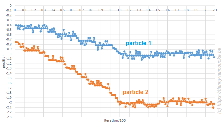
Monte Carlo in excel. A system of three particles on a line, with one particle fixed at 0. All particles interact through a Lennard-Jones potential. The Monte Carlo simulation shows how the particles move toward their equilibrium position.
The simplicity of Newton’s equations of motion make it possible to perform simple MD simulations, and already for a three particle system, you can see how unstable the algorithm is. Implementation of the leap-frog algorithm isn’t much more complex and shows incredible the stability of this algorithm. In the plot of the total energy you can even see how the algorithm fights back to retain stability (the spikes may seem large, but the same setup with a straight forward implementation of Newton’s equation of motion quickly moves to energies of the order of 100).
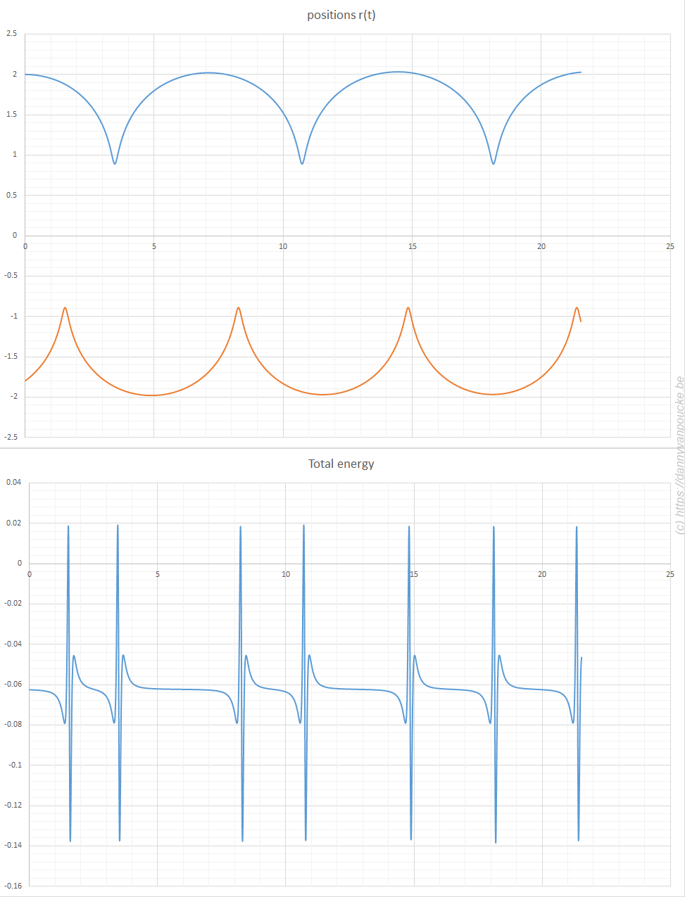
Molecular dynamics in excel. A system of three particles on a line, with one particle fixed at 0. All particles interact through a Lennard-Jones potential. The Molecular dynamics simulation shows how the particles move as time evolves. Their positions are updated using the leap-frog algorithm. The extreme hard nature of the Lennard-Jones potential gives rise to the sharp spikes in the total energy. It is this last aspect which causes the straight forward implementation of Newton’s equations of motion to fail.