Tag: theory and experiment
| Authors: |
Silviu Florin Acaru, Marc Comí, Panagiotis Falireas, Danny E. P. Vanpoucke, Richard Vendamme, and Katrien Bernaerts |
| Journal: |
Materials & Design 267, 116265 (2026) |
| doi: |
10.1016/j.matdes.2026.116265 |
| IF(2025): |
7.9 |
| export: |
bibtex |
| pdf: |
<Mat&Des_267> |
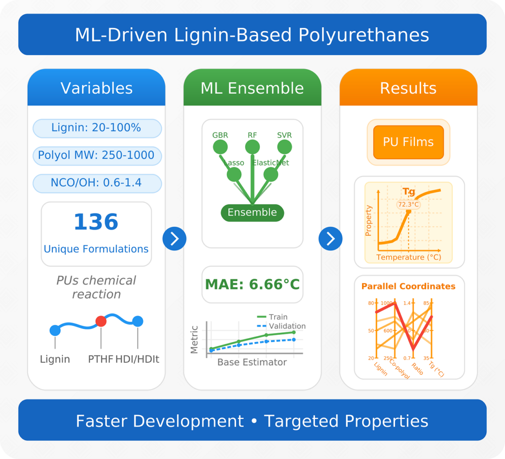 |
| Graphical Abstract: A machine learning ensemble accurately predicts glass transition temperatures for lignin-based polyurethanes within 6.66°C, despite being trained on a dataset of only 136 formulations. The model efficiently combines seven key features to overcome this data limitation. This optimized workflow generated over 4 million novel lignin-polyurethane formulations, with an intuitive interface accelerating the adoption of sustainable polyurethanes. |
Lignin-based polyurethanes (PUs) offer a compelling route towards sustainable material development, yet the challenge of designing chemical formulations with targeted properties, such as glass transition temperature (Tg), remains unresolved. In this work, we present a systematic approach, to explore key structural parameters—such as lignin content, polyol chain length, isocyanate functionality, and mixing ratios—across 136 unique formulations, creating a diverse dataset of ligninbased PUs. By harnessing this small dataset, we develop a machine learning (ML) ensemble model capable of accurately predicting Tg, with a mean absolute error of just 6.66°C on the validation set, surpassing the performance of conventional regression methods. Additionally, we enhance model interpretability by integrating advanced mapping techniques and employ an adaptive grid search algorithm to explore extrapolative scenarios. Our workflow, paired with a user-friendly interface, enables rapid discovery and optimization of formulations with desired properties. This study not only deepens the understanding of structure-property relationships in lignin-PUs but also provides a scalable ML-driven tool for designing sustainable materials with precision, highlighting the transformative potential of artificial intelligence in green chemistry and materials innovation.
Permanent link to this article: https://dannyvanpoucke.be/2026-paper_digiligninsylviu-en/
| Authors: |
Pieter Verding, Danny E.P. Vanpoucke, Yunus T. Aksoy, Tobias Corthouts, Maria R. Vetrano, and Wim Deferme |
| Journal: |
Adv. Mater. Technol. XX, YY (2025) |
| doi: |
10.1002/admt.202502104 |
| IF(2025): |
6.2 |
| export: |
bibtex |
| pdf: |
<AdvMaterTechnol_XX> |
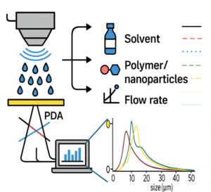 |
| Graphical Abstract: This study explores how machine learning models, trained on small experimental datasets obtained via Phase Doppler Anemometry (PDA), can accurately predict droplet size (D₃₂) in ultrasonic spray coating (USSC). By capturing the influence of ink complexity (solvent, polymer, nanoparticles), power, and flow rate, the model enables precise droplet control paving the way for optimized coatings in advanced functional materials. |
This study examines droplet formation in ultrasonic spray coating (USSC) as a function of ink formulation (solvent, polymer, nanoparticles). First, acetone with polyvinylidene fluoride (PVDF) at concentrations from 0-4.5 wt% is used to examine the effect of polymer additions. Additionally, acetone-based SiO2 nanofluids (0-10 g/L), are explored. Finally, the combination of both polymer (PVDF) and nanoparticles (SiO2) in acetone is studied. Droplet sizes are measured using Phase Doppler Anemometry under varying atomization power and flow rates. Machine Learning (ML) algorithms are employed to develop droplet size models from key spray parameters, including atomization power, flow rate, polymer concentration, and nanoparticle concentration. The model shows significantly higher accuracy than existing empirical models. The model is further validated on IPA-based inks with polyethylenimine (PEIE) or ZnO nanoparticles, and on acetone–cellulose acetate formulations, confirming its robustness across diverse ink systems. In addition to revealing the influence of coating parameters on the droplet formation and distribution, obtained both via experimental validation and ML, this study demonstrates that ML can be effectively applied to small experimental datasets, offering a robust framework for optimizing droplet formation and understanding key spray parameters in USSC for complex, unexplored inks enabling novel coating applications.
Permanent link to this article: https://dannyvanpoucke.be/2025-paper_mldroplets_pieterverding-en/
Today we had our fourth consortium meeting for the DigiLignin project. Things are moving along nicely, with a clear experimental database almost done by VITO, the Machine Learning model taking shape at UMaastricht, and quantum mechanical modeling providing some first insights.
Permanent link to this article: https://dannyvanpoucke.be/digilignin-c4-en/
| Authors: |
Kirill N. Boldyrev, Vadim S. Sedov, Danny E.P. Vanpoucke, Victor G. Ralchenko, & Boris N. Mavrin |
| Journal: |
Diam. Relat. Mater 126, 109049 (2022) |
| doi: |
10.1016/j.diamond.2022.109049 |
| IF(2020): |
3.315 |
| export: |
bibtex |
| pdf: |
<DRM> |
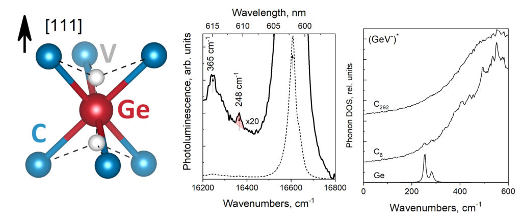 |
| Graphical Abstract: GeV split vacancy defect in diamond and the phonon modes near the ZPL. |
The vibrational behaviour of the germanium-vacancy (GeV) in diamond is studied through its photoluminescence spectrum and first-principles modeled partial phonon density of states. The former is measured in a region below 600 cm−1. The latter is calculated for the GeV center in its neutral, charged, and excited state. The photoluminescence spectrum presents a previously unobserved feature at 248 cm−1 in addition to the well-known peak at 365 cm−1. In our calculations, two localized modes, associated with the GeV center and six nearest carbon atoms (GeC6 cluster) are identified. These correspond to one vibration of the Ge ion along with the [111] orientation of the crystal and one perpendicular to this direction. We propose these modes to be assigned to the two features observed in the photoluminescence spectrum. The dependence of the energies of the localized modes on the GeV-center and their manifestation in experimental optical spectra is discussed.
Permanent link to this article: https://dannyvanpoucke.be/paper_gevpldft_vadim-en/
| Authors: |
Sergey Mitryukovskiy, Danny E. P. Vanpoucke, Yue Bai, Théo Hannotte, Mélanie Lavancier, Djamila Hourlier, Goedele Roos and Romain Peretti |
| Journal: |
Physical Chemistry Chemical Physics 24, 6107-6125 (2022) |
| doi: |
10.1039/D1CP03261E |
| IF(2020): |
3.676 |
| export: |
bibtex |
| pdf: |
<PCCP> |
 |
| Graphical Abstract: Comparison of the measured THz spectrum of 3 phases of Lactose-Monohydrate to the calculated spectra for several Lactose configurations with varying water content. |
The nanoscale structure of molecular assemblies plays a major role in many (µ)-biological mechanisms. Molecular crystals are one of the most simple of these assemblies and are widely used in a variety of applications from pharmaceuticals and agrochemicals, to nutraceuticals and cosmetics. The collective vibrations in such molecular crystals can be probed using terahertz spectroscopy, providing unique characteristic spectral fingerprints. However, the association of the spectral features to the crystal conformation, crystal phase and its environment is a difficult task. We present a combined computational-experimental study on the incorporation of water in lactose molecular crystals, and show how simulations can be used to associate spectral features in the THz region to crystal conformations and phases. Using periodic DFT simulations of lactose molecular crystals, the role of water in the observed lactose THz spectrum is clarified, presenting both direct and indirect contributions. A specific experimental setup is built to allow the controlled heating and corresponding dehydration of the sample, providing the monitoring of the crystal phase transformation dynamics. Besides the observation that lactose phases and phase transformation appear to be more complex than previously thought – including several crystal forms in a single phase and a non-negligible water content in the so-called anhydrous phase – we draw two main conclusions from this study. Firstly, THz modes are spread over more than one molecule and require periodic computation rather than a gas-phase one. Secondly, hydration water does not only play a perturbative role but also participates in the facilitation of the THz vibrations.
The 0.5 THz finger-print mode of alpha-lactose monohydrate.
Permanent link to this article: https://dannyvanpoucke.be/paper-lactosethz_romain-en/
| Authors: |
Dries De Sloovere, Danny E. P. Vanpoucke, Andreas Paulus, Bjorn Joos, Lavinia Calvi, Thomas Vranken, Gunter Reekmans, Peter Adriaensens, Nicolas Eshraghi, Abdelfattah Mahmoud, Frédéric Boschini, Mohammadhosein Safari, Marlies K. Van Bael, An Hardy |
| Journal: |
Advanced Energy and Sustainability Research 3(3), 2100159 (2022) |
| doi: |
10.1002/aesr.202100159 |
| IF(2022): |
?? |
| export: |
bibtex |
| pdf: |
<AdvEnSusRes> (OA) |
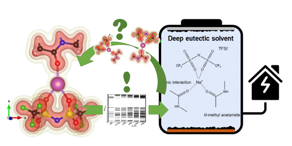 |
| Graphical Abstract: Understanding the electronic structure of Na-TFSI interacting with NMA. |
Sodium-ion batteries are alternatives for lithium-ion batteries in applications where cost-effectiveness is of primary concern, such as stationary energy storage. The stability of sodium-ion batteries is limited by the current generation of electrolytes, particularly at higher temperatures. Therefore, the search for an electrolyte which is stable at these temperatures is of utmost importance. Here, we introduce such an electrolyte using non-flammable deep eutectic solvents, consisting of sodium bis(trifluoromethane)sulfonimide (NaTFSI) dissolved in N-methyl acetamide (NMA). Increasing the NaTFSI concentration replaces NMA-NMA hydrogen bonds with strong ionic interactions between NMA, Na+, and TFSI–. These interactions lower NMA’s HOMO energy level compared to that of TFSI–, leading to an increased anodic stability (up to ~4.65 V vs Na+/Na). (Na3V2(PO4)2F3/CNT)/(Na2+xTi4O9/C) full cells show 74.8% capacity retention after 1000 cycles at 1 C and 55 °C, and 97.0% capacity retention after 250 cycles at 0.2 C and 55 °C. This is considerably higher than for (Na3V2(PO4)2F3/CNT)/(Na2+xTi4O9/C) full cells containing a conventional electrolyte. According to the electrochemical impedance analysis, the improved electrochemical stability is linked to the formation of more robust surface films at the electrode/electrolyte interface. The improved durability and safety highlight that deep eutectic solvents can be viable electrolyte alternatives for sodium-ion batteries.
Permanent link to this article: https://dannyvanpoucke.be/paper-desbatteries_dries-en/
| Authors: |
Rozita Rouzbahani, Shannon S.Nicley, Danny E.P.Vanpoucke, Fernando Lloret, Paulius Pobedinskas, Daniel Araujo, Ken Haenen |
| Journal: |
Carbon 172, 463-473 (2021) |
| doi: |
10.1016/j.carbon.2020.10.061 |
| IF(2019): |
8.821 |
| export: |
bibtex |
| pdf: |
<Carbon> |
 |
| Graphical Abstract: Artist impression of B incorporation during CVD growth of diamond. |
The methane concentration dependence of the plasma gas phase on surface morphology and boron incorporation in single crystal, boron-doped diamond deposition is experimentally and computationally investigated. Starting at 1%, an increase of the methane concentration results in an observable increase of the B-doping level up to 1.7×1021 cm−3, while the hole Hall carrier mobility decreases to 0.7±0.2 cm2 V−1 s−1. For B-doped SCD films grown at 1%, 2%, and 3% [CH4]/[H2], the electrical conductivity and mobility show no temperature-dependent behavior due to the metallic-like conduction mechanism occurring beyond the Mott transition. First principles calculations are used to investigate the origin of the increased boron incorporation. While the increased formation of growth centers directly related to the methane concentration does not significantly change the adsorption energy of boron at nearby sites, they dramatically increase the formation of missing H defects acting as preferential boron incorporation sites, indirectly increasing the boron incorporation. This not only indicates that the optimized methane concentration possesses a large potential for controlling the boron concentration levels in the diamond, but also enables optimization of the growth morphology. The calculations provide a route to understand impurity incorporation in diamond on a general level, of great importance for color center formation.
Permanent link to this article: https://dannyvanpoucke.be/paper_bdoping-en/
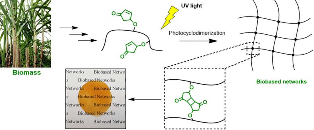 |
| Graphical Abstract: The formation of biobased polyacrylates. |
The controlled polymerization of a new biobased monomer, 4-oxocyclopent-2-en-1-yl acrylate (4CPA), was
established via reversible addition−fragmentation chain transfer (RAFT) (co)polymerization to yield polymers bearing pendent cyclopentenone units. 4CPA contains two reactive functionalities, namely, a vinyl group and an internal double bond, and is an unsymmetrical monomer. Therefore, competition between the internal double bond and the vinyl group eventually leads to gel formation. With RAFT polymerization, when aiming for a degree of polymerization (DP) of 100, maximum 4CPA conversions of the vinyl group between 19.0 and 45.2% were obtained without gel formation or extensive broadening of the dispersity. When the same conditions were applied in the copolymerization of 4CPA with lauryl acrylate (LA), methyl acrylate (MA), and isobornyl acrylate, 4CPA conversions of the vinyl group between 63 and 95% were reached. The additional functionality of 4CPA in copolymers was demonstrated by model studies with 4-oxocyclopent-2-en-1-yl acetate (1), which readily dimerized under UV light via [2 + 2] photocyclodimerization. First-principles quantum mechanical simulations supported the experimental observations made in NMR. Based on the calculated energetics and chemical shifts, a mixture of head-to-head and head-to-tail dimers of (1) were identified. Using the dimerization mechanism, solvent-cast LA and MA copolymers containing 30 mol % 4CPA were cross-linked under UV light to obtain thin films. The cross-linked films were characterized by dynamic scanning calorimetry, dynamic mechanical analysis, IR, and swelling experiments. This is the first case where 4CPA is described as a monomer for functional biobased polymers that can undergo additional UV curing via photodimerization.
Permanent link to this article: https://dannyvanpoucke.be/paper_nmrjules-en/
| Authors: |
Viraj Damle, Kaiqi Wu, Oreste De Luca, Natalia Ortí-Casañ, Neda Norouzi, Aryan Morita, Joop de Vries, Hans Kaper, Inge Zuhorn, Ulrich Eisel, Danny E.P. Vanpoucke, Petra Rudolf, and Romana Schirhagl, |
| Journal: |
Carbon 162, 1-12 (2020) |
| doi: |
10.1016/j.carbon.2020.01.115 |
| IF(2019): |
8.821 |
| export: |
bibtex |
| pdf: |
<Carbon> (Open Access) |
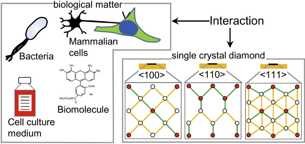 |
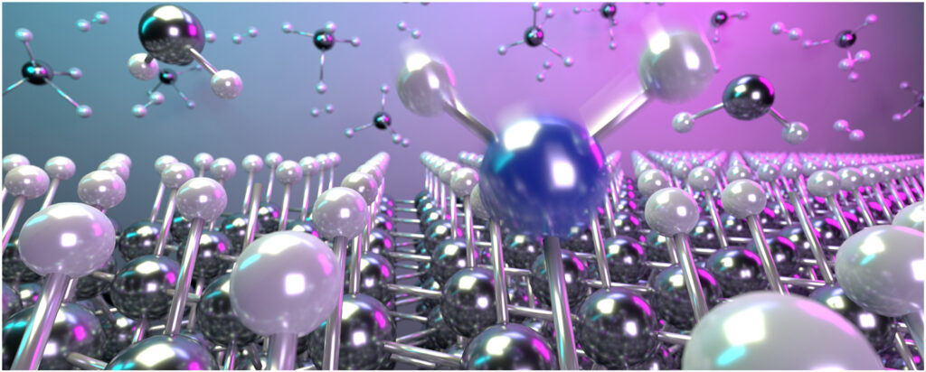
| Graphical Abstract: The preferential adsorption of biological matter on oriented diamond surfaces. |
Diamond has been a popular material for a variety of biological applications due to its favorable chemical, optical, mechanical and biocompatible properties. While the lattice orientation of crystalline material is known to alter the interaction between solids and biological materials, the effect of diamond’s crystal orientation on biological applications is completely unknown. Here, we experimentally evaluate the influence of the crystal orientation by investigating the interaction between the <100>, <110> and <111> surfaces of the single crystal diamond with biomolecules, cell culture medium, mammalian cells and bacteria. We show that the crystal orientation significantly alters these biological interactions. Most surprising is the two orders of magnitude difference in the number of bacteria adhering on <111> surface compared to <100> surface when both the surfaces were maintained under the same condition. We also observe differences in how small biomolecules attach to the surfaces. Neurons or HeLa cells on the other hand do not have clear preferences for either of the surfaces. To explain the observed differences, we theoretically estimated the surface charge for these three low index diamond surfaces and followed by the surface composition analysis using x-ray photoelectron spectroscopy (XPS). We conclude that the differences in negative surface charge, atomic composition and functional groups of the different surface orientations lead to significant variations in how the single crystal diamond surface interacts with the studied biological entities.
Permanent link to this article: https://dannyvanpoucke.be/paper_diamondromanaorientation2020-en/
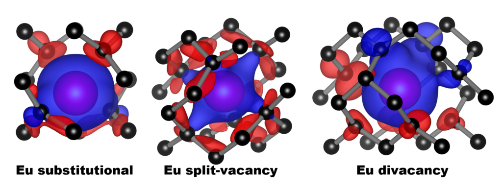 |
| Graphical Abstract: Spin polarization around the various Eu-defect models in diamond. Blue and red represent the up and down spin channels respectively. |
The incorporation of Eu into the diamond lattice is investigated in a combined theoretical-experimental study. The large size of the Eu ion induces a strain on the host lattice, which is minimal for the Eu-vacancy complex. The oxidation state of Eu is calculated to be 3+ for all defect models considered. In contrast, the total charge of the defect-complexes is shown to be negative: -1.5 to -2.3 electron. Hybrid-functional electronic-band-structures show the luminescence of the Eu defect to be strongly dependent on the local defect geometry. The 4-coordinated Eu substitutional dopant is the most promising candidate to present the typical Eu3+ luminescence, while the 6-coordinated Eu-vacancy complex is expected not to present any luminescent behaviour. Preliminary experimental results on the treatment of diamond �films with Eu-containing precursor indicate the possible incorporation of Eu into diamond �films treated by drop-casting. Changes in the PL spectrum, with the main luminescent peak shifting from approximately 614 nm to 611 nm after the growth plasma exposure, and the appearance of a shoulder peak at 625 nm indicate the potential incorporation. Drop-casting treatment with an electronegative polymer material was shown not to be necessary to observe the Eu signature following the plasma exposure, and increased the background
luminescence.
Permanent link to this article: https://dannyvanpoucke.be/paper_eudopingdrmspecial2018-en/


