| Authors: | Silviu Florin Acaru, Marc Comí, Panagiotis Falireas, Danny E. P. Vanpoucke, Richard Vendamme, and Katrien Bernaerts |
| Journal: | Materials & Design 267, 116265 (2026) |
| doi: | 10.1016/j.matdes.2026.116265 |
| IF(2025): | 7.9 |
| export: | bibtex |
| pdf: | <Mat&Des_267> |
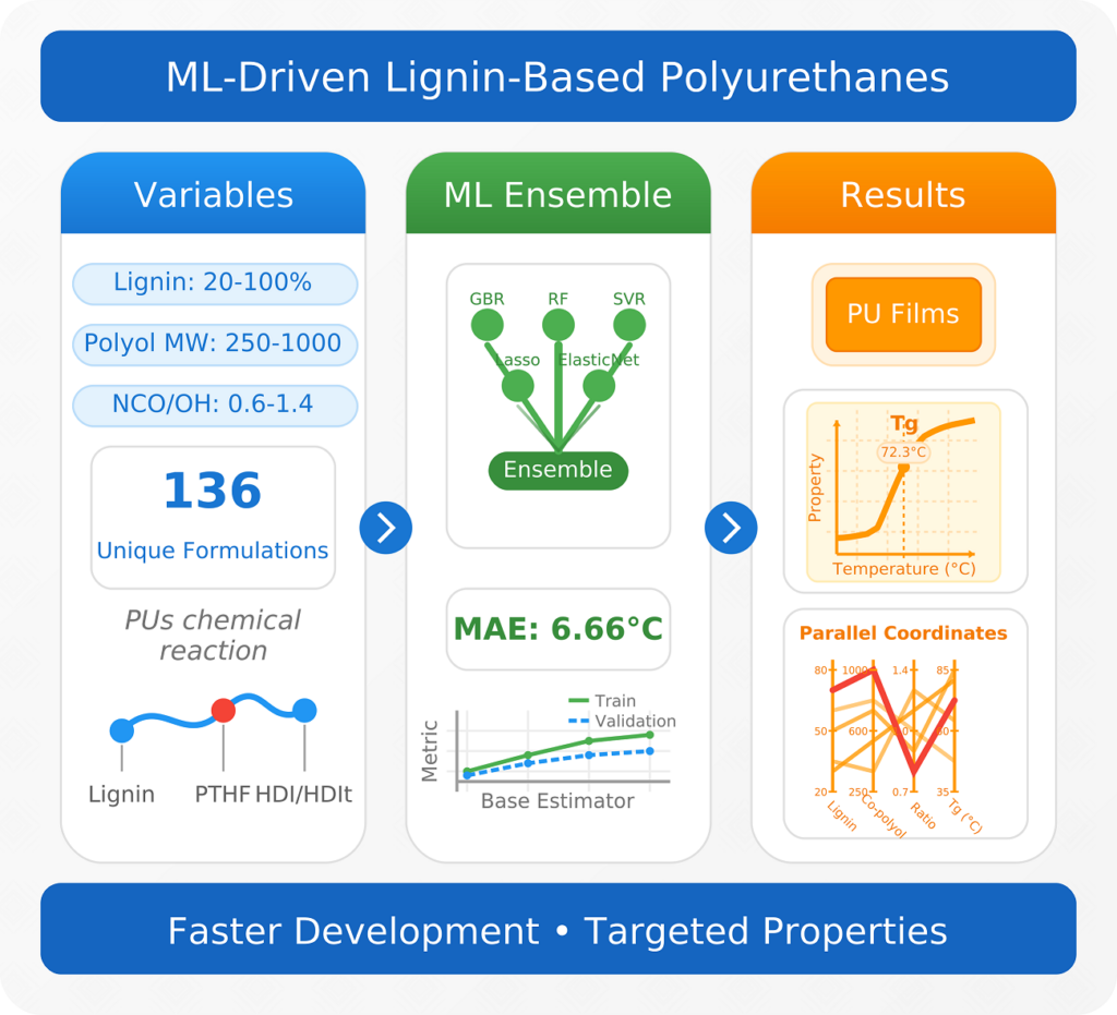 |
| Graphical Abstract: A machine learning ensemble accurately predicts glass transition temperatures for lignin-based polyurethanes within 6.66°C, despite being trained on a dataset of only 136 formulations. The model efficiently combines seven key features to overcome this data limitation. This optimized workflow generated over 4 million novel lignin-polyurethane formulations, with an intuitive interface accelerating the adoption of sustainable polyurethanes. |
Abstract
Lignin-based polyurethanes (PUs) offer a compelling route towards sustainable material development, yet the challenge of designing chemical formulations with targeted properties, such as glass transition temperature (Tg), remains unresolved. In this work, we present a systematic approach, to explore key structural parameters—such as lignin content, polyol chain length, isocyanate functionality, and mixing ratios—across 136 unique formulations, creating a diverse dataset of ligninbased PUs. By harnessing this small dataset, we develop a machine learning (ML) ensemble model capable of accurately predicting Tg, with a mean absolute error of just 6.66°C on the validation set, surpassing the performance of conventional regression methods. Additionally, we enhance model interpretability by integrating advanced mapping techniques and employ an adaptive grid search algorithm to explore extrapolative scenarios. Our workflow, paired with a user-friendly interface, enables rapid discovery and optimization of formulations with desired properties. This study not only deepens the understanding of structure-property relationships in lignin-PUs but also provides a scalable ML-driven tool for designing sustainable materials with precision, highlighting the transformative potential of artificial intelligence in green chemistry and materials innovation.