Recently, I decided to add a custom registration form to my website, as part of an effort to improve and streamline the “HIVE-STM tool experience” 😉 . Up until now, potential users had to directly send me an e-mail, telling me a bit more about themselves and their work. I would then e-mail them the program, and add their information to a user list for future reference (i.e., support and some statistics for my personal entertainment).
This has the drawback that any future user needs to wait until I find the time to reply. To improve on the user-friendliness, I thought it would be nice to automate this a bit. A first step in this process entails making the application a bit more uniform: using an online registration form.
The art of learning something new: Do it from scratch
 What started out with the intention of being an almost trivial exercise in building a web-form, turned into a steep learning curve about web-development and cyber-security. I am aware there exists many tools which generate forms for websites or even provide you a platform which hosts the form (e.g., google-forms, which I used in the past), but I wanted to do implement it myself (…something to do with pride 😉 ). Having build websites using HTML and CSS in the past, and having some basic experience with Javascript, this looked like a fun afternoon project. The HTML for the form was easily created using the tutorials found on w3schools.com and an old second edition “Handboek HTML5 en CSS3“, I picked up a few years ago browsing a second hand bookshop. Trouble, however, started rearing its ugly head as soon as I wanted to integrate this form in this WordPress website. Just pasting this into a page or post doesn’t really work, as WordPress wants to “help” you, and prevent you from hurting yourself. This is a fantastic feature if you have no clue about HTML/CSS/… or don’t want to care about it. Unfortunately, if you want to do something slightly more advanced you are in for a hell of a ride, as you find out the relevant bits get redacted or disabled.
Searching for specific solutions with regard to creating a custom form in WordPress I was astounded at how often the default suggestion is: “use plugin XXX” or “use tool YYY”. Are we loosing the ability to want to craft something ourselves? Yes of course, there are professional tools available which can be better than anything you yourself can build in a short amount of time…but should it discourage you of trying, and feeling the satisfaction of having created something? I digress.
In the end, I discovered a good quality tutorial (once you get past the reasons why not to do it) and I started a long uphill battle trying to bend WordPress to my will:
- Paste form-code in post ⇒ WP countermove: remove relevant tags essentially killing the form.
- Solution: put the form in a dedicated template ⇒ WP countermove: hard to integrate in existing theme, will be removed upon update of the theme
- Solution: create a child-theme ⇒ WP countermove: interesting exercise is getting the CSS style-sheet to work together with that of the parent theme. (wp_enqueue_style, wp_enqueue_scripts, get_template_directory_uri() and get_stylesheet_directory_uri() saved the day.)
- Add PHP back-end to the form…and deal with the idiosyncrasies of this scripting language. Crashed the website a few time due to missing “;”… error messages would be nice, instead of the blank web-page.
Trying not to torture future users
At this point, the form accepted input, and collected it via the PHP $_POST global variable. En route to this point, I read quite a few warnings about Cross-Site Request Forgery (CSRF) and that one should protect against it. Luckily, the tutorial practically showed how to do this in WordPress using nonces…in contrast to WordPress theme handbook which gives in formation, but not easy to understand if you are new to the subject.
With a basic sense of security, I was aiming at making things user-friendly, i.e., if something goes wrong it would be nice if you do not need to again fill out the form entirely. Searching for ways to keep this information I came across a lot of options, none of which seemed to work (cookies, PHP variables, global variables, etc). The problem appeared to originate from the fact that the information was not persistent. Once the web page started reloading, everything got erased. It was only at this point that I learned about “transients” in WordPress, and using get_transient() and set_transient() resolved all the issues instantaneously. There is only one caveat at this point: If two potential users submit their registration at almost the same time one may end up seeing the registration information of the other. (However, at this time the program is far from famous enough to present any issues, so statistics will save us from this).
Only one thing remained to be done: put all relevant information into two e-mail messages, one to be sent to myself, and one to be sent to the potential user. For this, I made use of the PHP mail() function. It works quite nicely, and after playing around with it for a bit (and convincing myself a nice HTML formatted layout will not work for example in gmail) the setup was complete. That evening, I went to bed, happy with the accomplishment: I had created something.
Too popular for comfort
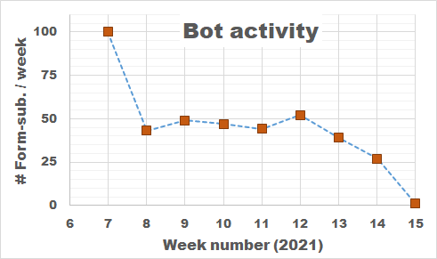
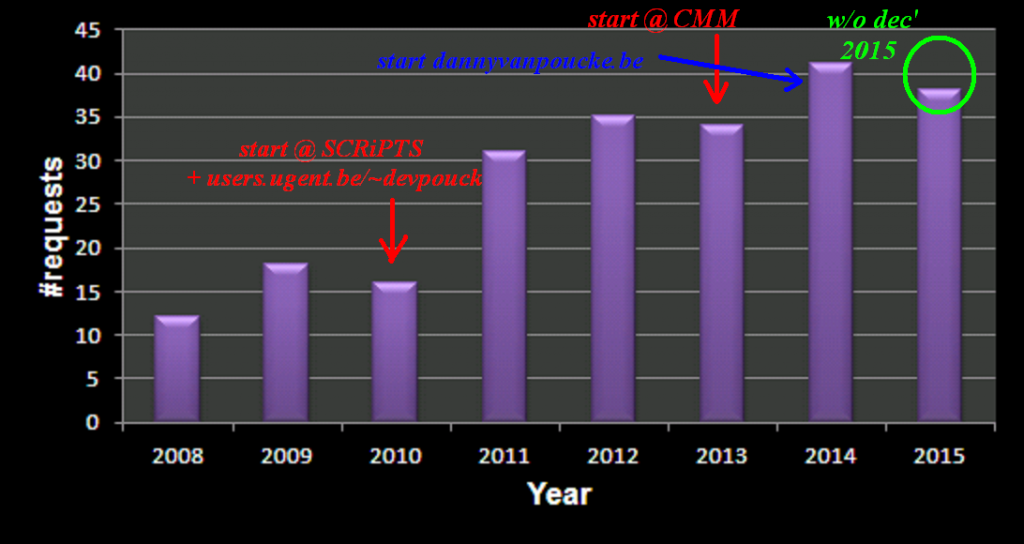
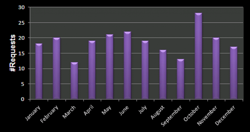
Bot Activity on the HIVE registration form during February and March of 2021.
The next morning, I was amazed to find already several applications for the HIVE-STM program in my mailbox (that is, in addition to my own test runs). These were not sent by real humans, but appeared to be the work of bots just filling out the form and sending it off. This left me a bit puzzled, and I have been looking for the reason why anyone would actually bother writing a bot for this purpose. So far I’ve seen the suggestion that this is to improve the SEO of websites, generate spam-email (to yourself or with you as middleman), DOS-attacks, get access to your SQL database via code injection,…and after all my searches, I start to get the impression this may also be a means of promoting all the plugins, tools, frameworks that block these bots? In roughly each discussion you find, there will be at least one person promoting such a foolproof perfect tool 😯 🙄 …but might just be me.
So how do we deal with these bots, preferably without driving potential users crazy? Reading all the suggestions (which unfortunately provide extremely little information on the actual working and logic of spam-bots themselves) I added, in several rounds, some tricks to block/catch the bots, and have been tracking the submits since the form went live. As you can see there is a steady stream of some 50 bots weekly trying to fill out the form. The higher number in the first week is due to any submission being redirected to the original form page, as such the same bots performed multiple attempts within the time-range of a few minutes. In about two months, I collected the results of 400 registration attempts by bots (and 4 by humans).
Analyzing the results, I learned learned some interesting things.
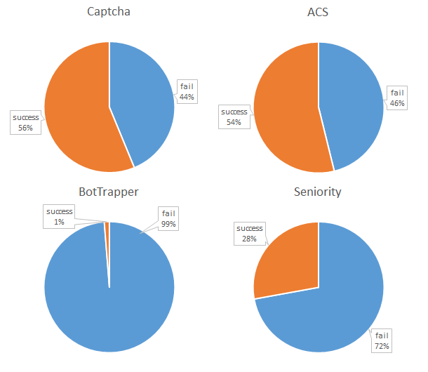
How to catch a bot? I track 4 different signals which may be indicative of bot behavior.
1. To Captcha or not to Captcha?
One of the first things to add, from a human perspective is “a captcha”. The captcha is manually implemented simple random sum/product/subtraction. It should be easy for humans, but it is annoying as they need to fill out an extra field (and may fill it out incorrectly). Interestingly, 56% of the bots fill out the Captcha correctly. Of course more complicated versions could be implemented or used…but the bottom line is simple: it generally does not do the job, and annoys the actual human being.
2. Bot Trapping for furs?
Going beyond captcha’s, a lot of tutorials suggest the use of a honeypot. One can either make use of automated options of existing frameworks, plugins or …implement these oneself. This option appears to be very successful in targeting bots. The 1% successful cases coincided with the only human submissions. At this point we appear to have a “fool-proof” method for distinguishing between humans and bots.
3. Dropping the bot down the box?
Interestingly, drop-down menu’s with not generally used topics seem to throw off bots as well. The seniority drop-down menu shows failure rates even better than the captcha.
Conclusion
Writing your own form from scratch is a very interesting exercise, and well worth the time if you want to learn more about web-security as well as the inner workings of the framework used for your website. Bots are an interesting nuisance, and captcha’s just bother your user as most bots can easily deal with them. Logging the inputs of the bots does show a wide range in quality of these bots. Some just fill out garbage, while others appear to be quite smart, filling out reasonable answers. Other bots clearly have malignant purposes, which becomes clear from the code they try to plug into the form fields.
For now, the registration form seems to be able to distinguish between human-and bot-users. As such, we have successfully completed another step in upgrading the STM-program.
 The first PC we got at our home was a
  Where in 2005 you bought a single CPU with a high clock rate, you now get a machine with multiple cores. Most machines you can get these days have a minimum of 2 cores, with quad-core machines becoming more and more common. But, there is always a but, even though you now have access to multiple times the processing power of 2005, this does not mean that your own code will be able to use it. Unfortunately there is no simple compiler switch which makes your code parallel (like the -m64 switch which
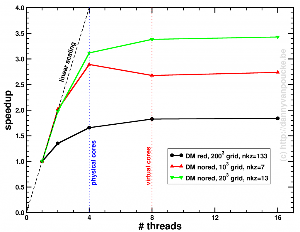
 and the circumference and surface area of a disc. We will be looking at a rather large disc, one with a radius equal to the distance between the sun, and the nearest star,
  (or
(or  km ). As a single precision variable
  or
or  m² ) to within 1 m². Even the surface of a disc the size of our milky way could be calculated with an accuracy of a few hundred square km (or ± the size of Belgium ).