

Over the past few weeks I have bumped into several issues each tracing back to numerical accuracy. Although I have been programming for almost two decades I never had to worry much about this, making these events seem as-if the universe is trying to tell me something.
Now, let me try to give a proper start to this story; Computational (materials) research is generally perceived as a subset of theoretical (materials) research, and it is true that such a case can be made. It is, however, also true that such thinking can trap us (i.e. the average computational physicist/chemist/mathematician/… programming his/her own code) with numerical accuracy problems. While theoretical equations use exact values for numbers, a computer program is limited by the numerical precision of the variables (e.g. single, double or quadruple precision for real numbers) used in the program. This means that actual numbers with a larger precision are truncated or rounded to the precision of the variable (e.g. 1/3 becomes 0.3333333 instead of 0.333… with an infinite series of 3’s). Most of the time, this is sufficient, and nothing strange will happen. Even more, most of the time, the additional digits would only increase the computational cost while not improving the results in a significant fashion.
Interstellar disc
To understand the importance, or the lack thereof, of additional significant digits, let us first have a look at the precision of 


Knowing this, our mind is quickly put at easy regarding possible issues regarding numerical accuracy. However, once in a while we run into one exceptional case (or three, in my case).
1. Infinitesimal finite elements
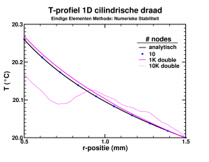
Temperature profile in the insulating layer of a cylindrical wire.
While looking into the theory behind finite elements, I had some fun implementing a simple program which calculated the temperature distribution due to heat transport in an insulating layer. The finite element approach performed rather nicely, leading to good approximate results, already for a few dozen elements. However, I wanted to push the implementation a bit (the limit of infinite elements should give the exact solution). Since the set of equations was solved by a LAPACK subroutine, using 10 000 elements instead of 10 barely impacted the required time (writing the results took most of 2-3 seconds anyway). The results on the other hand were quite funny as you can see in the picture. The initial implementation, with single precision variables, breaks down even worse already at 1000 elements. Apparently the elements had become too small leading to too small variations of the properties in the stiffness-matrix, resulting in the LAPACK subroutine returning nonsense.
So it turns out that you can have too many elements in a finite elements method.
2. Small volumes: A few more digits please
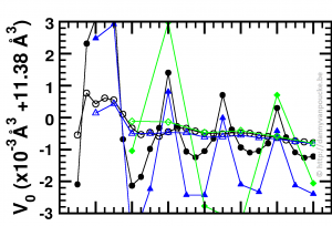
Optimized volume in Equation of State fit, as function of the range of the fitting data, and step size between data-points. green diamonds, blue triangles and black discs: 1% , 0.5% and 0.25% volume steps respectively.
Recently, I started working at the Wide Band Gap Materials group at the University of Hasselt. So in addition to MOFs I am also working on diamond based materials. While setting up a series of reference calculations, using scripts which already suited me well during my work on MOFs, I was trying to figure out for which volume range, and step size I would get a sufficient convergence in my Equation-of-States Fitting procedure. For the MOFs this is a computationally rather expensive (and tedious) exercise, which, fortunately, gives clear results. For the 2-atom diamond unit cell the calculations are ridiculously fast (in comparison), but the results were confusing. As you can see in the picture, the values I obtained from the different fits seem to oscillate. Checking my E(V) data showed nothing out of the ordinary. All energies and volumes were clearly distinguishable, with the energies given with a precision of 0.001 meV, and the volumes with a precision of 0.01 Å3. However, as you can see in the figure, the volume-oscillations are of the order of 0.001 Å3, ten times smaller than our input precision. Calculating the volumes based on the lattice parameters to get a precision of 10-6 Å3 for the input volumes stabilizes the convergence behavior of the fits (open symbols in the figure). This problem was not present with the MOFs since these have a unit cell volume which is one hundred times larger, so a precision of 0.01 Å3 makes the relative error on the volumes one hundred times smaller than was the case for diamond.
In essence, I was trying to get more accurate output than the input I provided, which will never give sensible results (even if they actually look sensible).
3. Many grains of sand really start to pile up after a while
The last one is a bit embarrassing as it lead to a bug in the HIVE-toolbox, which is fixed in the mean time.
One of the HIVE-toolbox users informed me that the dosgrabber routine had crashed because it could not find the Fermi-level in the output of a VASP calculation. Although VASP itself gives a value for the Fermi-level, I do not use it in the above sub-program, since this value tend to be incorrect for spin-polarized systems with different minority and majority spins. However, in an attempt to be smart (and efficient) I ended up in trouble. The basic idea behind my Fermi-level search is just running through the entire Density of States-spectrum until you have counted for all the electrons in the system. Because the VASP estimate for the Fermi-level is not that far of, you do not need to run through the entire list of several thousand entries, but you could just take a subset-centered around the estimated Fermi-level and check in that subset, speeding this up by a factor of 10 to 100. Unfortunately I calculated the energy step size between density of states entries as the difference between the first two entries, which are given to with an accuracy of 0.001 eV. I guess you already have a feeling what will be the problem. When the index of the estimated Fermi-level is 1000, the error will be of the order of 1 eV, which is much larger than the range I took into account. Fortunately, the problem is easily solved by calculating the energy step size as the difference between the first and last index, and divide by the number of steps, making the error in the particular case more than a thousand times smaller.
So, trying to be smart, you always need to make sure you really are being smart, and remember that small number can become very big when there are a lot of them.