It could be that I’ve perhaps found out a little bit about the structure
of atoms. You must not tell anyone anything about it. . .
–Niels Bohr (1885 – 1965),
in a letter to his brother (1912)
Getting the news that a paper got accepted for publication is exciting news, but it can also be a little bit sad since it indicates the end of a project. Little over a month ago we got this great news regarding our paper for the journal of chemical information and modeling. It was the culmination of a side project Goedele Roos and I had been working on, in an on-and-off fashion, over the last two years.
When we started the project each of us had his/her own goal in mind. In my case, it was my interest in showing that my Hirshfeld-I code could handle systems which are huge from the quantum mechanical calculation point of view. Goedele, on the other hand, was interested to see how good Hirshfeld-I charges behaved with increasing size of a molecular fraction. This is of interest for multiscale modeling approaches, for which Martin Karplus, Michael Levitt, and Arieh Warshel got the Nobel prize in chemistry in 2013. In such an approach, a large system, for example a solvated biomolecule containing tens of thousands of atoms, is split into several regions. The smallest central region, containing the part of the molecule one is interested in is studied quantum mechanically, and generally contains a few dozen up to a few hundred atoms. The second shell is much larger, and is described by force-field approaches (i.e. Newtonian mechanics) and can contain ten of thousands of atoms. Even further from the quantum mechanically treated core a third region is described by continuum models.
What about the behavior of the charges? In a quantum mechanical approach, even though we still speak of electrons as-if referring to classical objects, we cannot point to a specific point in space to indicate: “There it is”. We only have a probability distribution in space indicating where the electron may be. As such, it also becomes hard to pinpoint an atom, and in an absolute sense measure/calculate it’s charge. However, because such concepts are so much more intuitive, many chemists and physicists have developed methods, with varying success, to split the electron probability distribution into atoms again. When applying such a scheme on the probability distributions of fractions of a large biomolecule, we would like the atoms at the center not to change to much when the fraction is made larger (i.e. contain more atoms). This would indicate that from some point onward you have included all atoms that interact with the central atoms. I think, you can already see the parallel with the multiscale modeling approach mentioned above; where that point would indicate the boundary between the quantum mechanical and the Newtonian shell.
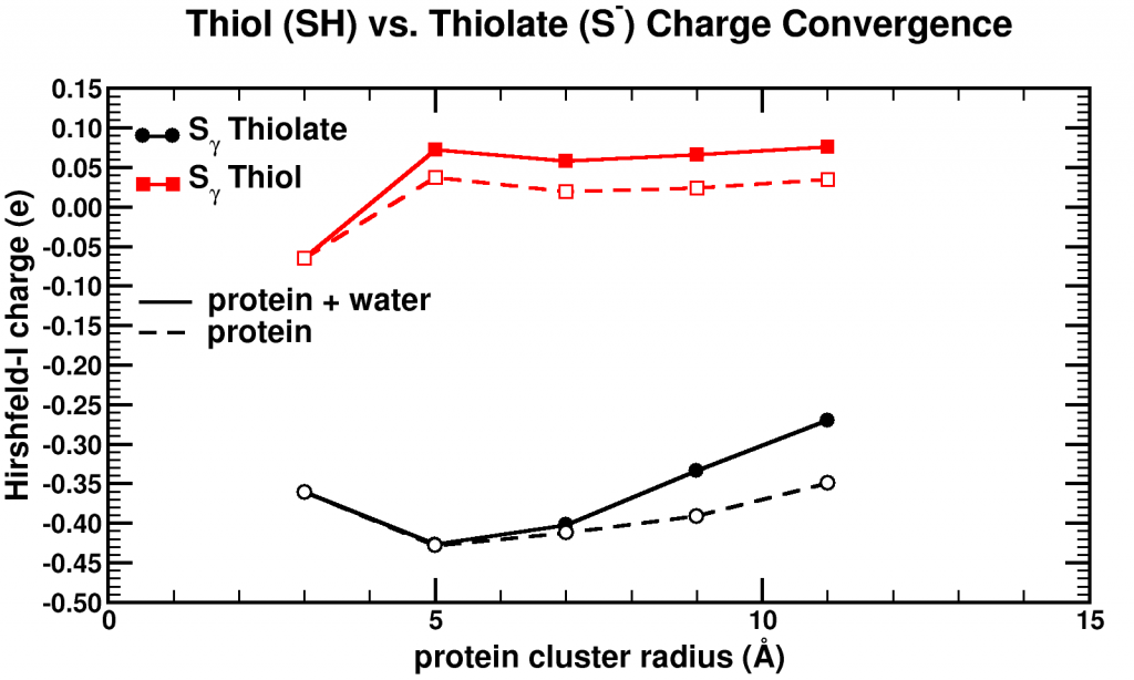
Convergence of Hirshfeld-I charges for clusters of varying size of a biomolecule. The black curves show the charge convergence of an active S atom, while the red curves indicate a deactivated S atom.
Although, we expected to merely be studying this convergence behavior, for the particular partitioning scheme I had implemented, we dug up an unexpected treasure. Of the set of central atoms we were interested all except one showed the nice (and boring) convergence behavior. The exception (a sulfur atom) showed a clear lack of convergence, it didn’t even show any intend toward convergence behavior even for our system containing almost 1000 atoms. However, unlike the other atoms we were checking, this S atom had a special role in the biomolecule: it was an active site, i.e. the atom where chemical reactions of the biomolecule with whatever else of molecule/atom are expected to occur.
Because this S atom had a formal charge of -1, we bound a H atom to it, and investigated this set of new fractions. In this case, the S atom, with the H atom bound to it, was no longer an active site. Lo and behold, the S atom shows perfect convergence like all other atoms of the central cluster. This shows us that an active site is more than an atom sitting at the right place at the right time. It is an atom which is reaching out to the world, interacting with other atoms over a very long range, drawing them in (>10 ångström=1 nm is very far on the atomic scale, imagine it like being able to touch someone who is standing >20 m away from you). Unfortunately, this is rather bad news for multiscale modeling, since this means that if you want to describe such an active site accurately you will need an extremely large central quantum mechanical region. When the active site is deactivated, on the other hand, a radius of ~0.5 nm around the deactivated site is already sufficient.
Similar to Bohr, I have the feeling that “It could be that I’ve perhaps found out a little bit about the structure
of atoms.”, and it makes me happy.


