Tag: tools

Animated Primes

Optimus Prime

Optimus Prime, the most prime of all autobots.[source]

2, 3, 5, 7, 11, 13, 17, 19, 23, …and on toward infinity. Prime numbers are a part of mathematics which seduce most of us at some point in our lives to try and “solve them”. There is structure in them, but too little to be easily understandable, and too much to let go and consider them chaos.

Recently, my girlfriend got sucked into this madness. Luckily she is not trying to generate the next largest prime (which would need to have more than 22 Million digits, although I might have jinxed it now). Instead she is looking for order into chaos; leading to pen and paper graphs, evolving into excel worksheets being abused as ordinary bitmap pictures and finally mathematica applications for even more heavy lifting.

These last exercises came to a somewhat grinding halt when mathematica refused to generate a gif-animation (it just failed to do the job without providing any warning that something might have gone awry). However, because it could generate the separate frames without any issues, I was tempted to dig up an old fortran module which allowed me to generate gif images and animations. I remembered correctly that it was able to both read and write gif-images, and so, after 10 minutes of writing a small program (9 minutes remembering how things worked) and another 10 linking in all dependencies and fixing some inconsistencies, I had a working program for generating a gif animation from separate gif images.

Animated gif, generated in fortran.

The initial test went smoothly. Using some simple gif images I created in paint, the resulting 4 frame animation is the one on the left (which is probably giving you a headache as you read this ;-).

The real test, with the single frame gifs Sylvia had prepared, was rather interesting: It failed miserably. Fortunately it also taught us the origin of the problem: mathematica was generating frames of different dimensions. And although this does not give rise to problems in the workbook or generated avi, it does kill an animated gif. After fixing this, also mathematica successfully generated the animated gif Sylvia wanted to see. Also my own small program was now able to perform the intended trick, although it showed that a different color-map was created for each frame by mathematica, something my own implementation did not handle well (we’ll fix that somewhere in the future).

The executable (including prerequisite dll’s) can be downloaded here.

If you do not suffer from epileptic seizures (or not yet), you could check out the results in the spoiler below.

Spoiler Inside: gif-animations SelectShow

Virtual Winterschool 2016: Computational Solid State Physics & Chemistry

In just an hour, I’ll be presenting my talk at the virtual winterschool 2016. In an attempt to tempt fate as much as possible I will try to give/run real-time examples on our HPC in Gent, however at this moment no nodes are available yet to do so. Let’s keep our fingers crossed and see if it all works out.

Abstract

Modern materials research has evolved to the point where it is now common practice to manipulate materials at nanometer scale or even at the atomic scale (e.g. Intel’s skylake architecture with 14nm features, atomic layer deposition and surface structure manipulations with an STM-tip). At these scales, quantum mechanical effects become ever more relevant, making their prediction important for the field of materials science.

In this session, we will discuss how advanced quantum mechanical calculations can be performed for solids and indicate some differences with standard quantum chemical approaches. We will touch upon the relevant concepts for performing such calculations (plane-wave basis-sets, pseudo-potentials, periodic boundary conditions,…) and show how the basic calculations are performed with the VASP-code. You will familiarize yourself with the required input files and we will discuss several of the most important output-files and the data they contain.

At the end of this session you should be able to set up a single-point calculation, a structure optimization, a density of states and band structure calculation.

Additional Files/Info

HIVE-STM: A simple post-processing tool for simulating STM

While I was working on my PhD-thesis on Pt nanowires at the university of Twente, one of the things I needed was a method for simulating scanning-tunneling microscopy (STM) images in a quick and easy way. This was because the main experimental information on on these nanowires was contained in STM-images.

Because I love programming, I ended up writing a Delphi-program for this task. Delphi, being an Object Oriented version of the Pascal-programming language containing a Visual Components Library, was ideally suited for writing an easy to use program with a graphical user interface (GUI). The resulting STM-program was specifically designed for my personal needs and the system I was working on at that time.

In August 2008, I was contacted by two German PhD students, with the request if it would be possible for them to use my STM program. In October, an American post-doc and a South-Korean graduate student followed with similar requests, from which point onward I started getting more and more requests from researchers from all over the world. Now, seven years later, I decided to put all “HIVE-users” in a small data-base just to keep track of their number and their affiliation. I already knew I send the program to quite a lot of people, but I was still amazed to discover that it were 225 people from 34 countries.

Hive Requests December 2015

Bar-graph showing the evolution in requests for the HIVE-STM program.

There is a slow but steady increase in requests over the years, with currently on average about one request every week. It is also funny to see there was a slight setback in requests both times I started in a new research-group. For 2015, the data is incomplete, as it does not include all requests of the month December. Another way to distribute the requests is by the month of the year. This is a very interesting graph, since it clearly shows the start of the academic year (October). There are two clear minima (March and September), for which the later is probably related due to the fact that it is the last month of before the start of the academic year (much preparation for new courses) and, in case of the solid state community, this month is also filled with conferences. The reason why there is a minimum in March, however, escapes me ( 💡 all suggestions are welcome 💡 ).

Hive requests per month.

Distribution of requests for the HIVE-STM program on a monthly basis.

The geographic distribution of affiliations of those requesting the STM-program shows Europe, Azia and America to take roughly equal shares, while African affiliations are missing entirety. Hopefully this will change after the workshop on visualization and analysis of VASP outputs delivered at the Center for High Performance Computing‘s 9th National Meeting in South Africa by Dr. David Carballal. By far the most requests come from the USA (57), followed by China(23) and then Germany(15). South-Korea(14) unexpectedly takes the fourth place, while the fifth place is a tie between the UK, Spain and India(12 each).

Hive requests demographics 2015

Distribution of Hive requests per country and continent.

All in all, the STM program seems to be of interest to many more researchers than I would have ever expected, and has currently been cited about 25 times, so it is time to add a page listing these papers as examples of what can be done with HIVE(which has in the mean time been done, check out useful link n°2).

Happy Hiving to all of you, and thank you for your trust.


Useful link:
[1] More information on the HIVE-STM program and how to acquire it.

[2] List of publications using and citing the HIVE-STM program.

Fortran dll’s and libraries: a Progress bar

In the previous fortran tutorials, we learned the initial aspects of object oriented programming (OOP) in fortran 2003. And even though our agent-based opinion-dynamics-code is rather simple, it can quickly take several minutes for a single run of the program to finish. Two tools which quickly become of interest for codes that need more than a few minutes to run are: (1) a progress bar, to track the advance of the “slow” part of the code and prevent you from killing the program 5 seconds before it is to finish, and (2) a timer, allowing you to calculate the time needed to complete certain sections of code, and possibly make predictions of the expected total time of execution.

In this tutorial, we will focus on the progress bar. Since our (hypothetical) code is intended to run on High-Performance Computing (HPC) systems and is written in the fortran language, there generally is no (or no easy) access to GUI’s. So we need our progress bar class to run in a command line user interface. Furthermore, because it is such a widely useful tool we want to build it into a (shared) library (or dll in windows).progress_1pct

The progress bar class

What do we want out of our progress bar? It needs to be easy to use, flexible and smart enough to work nicely even for a lazy user. The output it should provide is formatted as follows: <string> <% progress> <text progress bar>, where the string is a custom character string provided by the user, while ‘%progress’ and ‘text progress bar’ both show the progress. The first shows the progress as an updating number (fine grained), while the second shows it visually as a growing bar (coarse grained).

  1. type, public :: TProgressBar
  2. private
  3. logical :: init
  4. logical :: running
  5. logical :: done
  6. character(len=255) :: message
  7. character(len=30) :: progressString
  8. character(len=20) :: bar
  9. real :: progress
  10. contains
  11. private
  12. procedure,pass(this),public :: initialize
  13. procedure,pass(this),public :: reset
  14. procedure,pass(this),public :: run
  15. procedure,pass(this),private:: printbar
  16. procedure,pass(this),private:: updateBar
  17. end type TProgressBar

All properties of the class are private (data hiding), and only 3 procedures are available to the user: initialize, run and reset. The procedures, printbar and updatebar are private, because we intend the class to be smart enough to decide if a new print and/or update is required. The reset procedure is intended to reset all properties of the class. Although one might consider to make this procedure private as well, it may be useful to allow the user to reset a progress bar in mid progress.(The same goes for the initialize procedure.)

  1. subroutine run(this,pct,Ix,msg)
  2. class(TProgressBar) :: this
  3. real::pct
  4. integer, intent(in), optional :: Ix
  5. character(len=*),intent(in),optional :: msg
  6.  
  7. if (.not. this%init) call this%initialize(msg)
  8. if (.not. this%done) then
  9. this%running=.true.
  10. this%progress=pct
  11. call this%updateBar(Ix)
  12. call this%printbar()
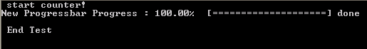
  13. if (abs(pct-100.0)<1.0E-6) then
  14. this%done=.true.
  15. write(*,'(A6)') "] done"
  16. end if
  17. end if
  18.  
  19. end subroutine run

In practice, the run procedure is the heart of the class, and the only procedure needed in most applications. It takes 3 parameters: The progress (pct), the number of digits to print of pct (Ix),and the <string> message (msg). The later two parameters are even optional, since msg may already have been provided if the initialize procedure was called by the user. If the class was not yet initialized it will be done at the start of the procedure. And while the progress bar has not yet reached 100% (within 1 millionth of a %) updates and prints of the bar are performed. Using a set of Boolean properties (init, running, done), the class keeps track of its status. The update and print procedures just do this: update the progress bar data and print the progress bar. To print the progress bar time and time again on the same line, we need to make use of the carriage return character (character 13 of the ASCII table):

write(*,trim(fm), advance='NO') achar(13), trim(this%message),trim(adjustl(this%progressString)),'%','[',trim(adjustl(this%bar))

The advance=’NO‘ option prevents the write statement to move to the next line. This can sometimes have the unwanted side-effect that the write statement above does not appear on the screen. To force this, we can use the fortran 2003 statement flush(OUTPUT_UNIT), where “OUTPUT_UNIT” is a constant defined in the intrinsic fortran 2003 module iso_fortran_env. For older versions of fortran, several compilers provided a (non standard) flush subroutine that could be called to perform the same action. As such, we now have our class ready to be used. The only thing left to do is to turn it into a dll or shared library.progress_25pct

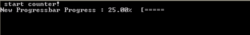
How to create a library and use it

There are two types of libraries: static and dynamic.

Static libraries are used to provide access to functions/subroutines at compile time to the library user. These functions/subroutines are then included in the executable that is being build. In linux environments these will have the extension “.a”, with the .a referring to archive. In a windows environment the extension is “.lib”, for library.

Dynamic libraries are used to provide access to functions/subroutines at run time. In contrast to static libraries, the functions are not included in the executable, making it smaller in size. In linux environments these will have the extension “.so”, with the .so referring to shared object. In a windows environment the extension is “.dll”, for dynamically linked library.

In contrast to C/C++, there is relatively little information to be found on the implementation and use of libraries in fortran. This may be the reason why many available fortran-“libraries” are not really libraries, in the sense meant here. Instead they are just one or more files of fortran code shared by their author(s), and there is nothing wrong with that. These files can then be compiled and used as any other module file.

So how do we create a library from our Progressbar class? Standard examples start from a set of procedures one wants to put in a library. These procedures are put into a .f or .f90 file. Although they are not put into a module (probably due to the idea of having compatibility with fortran 77) which is required for our class, this is not really an issue. The same goes for the .f03 or .f2003 extension for our file containing a fortran 2003 class. To have access to our class and its procedures in our test program, we just need to add the use progressbarsmodule clause. This is because our procedures and class are incorporated in a module (in contrast to the standard examples). Some of the examples I found online also include compiler dependent pragmas to export and import procedures from a dll. Since I am using gfortran+CB for development, and ifort for creating production code, I prefer to avoid such approaches since it hampers workflow and introduces another possible source of bugs.

The compiler setups I present below should not be considered perfect, exhaustive or fool-proof, they are just the ones that work fine for me. I am, however, always very interested in hearing other approaches and fixes in the comments.
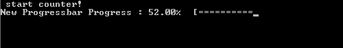
progress_52pct

Windows

The windows approach is very easy. We let Code::Blocks do all the hard work.

shared library: PBar.dll

Creating the dll : Start a new project, and select the option “Fortran DLL“. Follow the instructions, which are similar to the setup of a standard fortran executable. Modify/replace/add the fortran source you wish to include into your library and build your code (you can not run it since it is a library).

Creating a user program : The program in which you will be using the dll is setup in the usual way. And to get the compilation running smoothly the following steps are required:

  • Add the use myspecificdllmodule clause where needed, with myspecificdllmodule the name of the module included in the dll you wish to use at that specific point.
  • If there are modules included in the dll, the *.mod files need to be present for the compiler to access upon compilation of the user program. (Which results in a limitation with regard to distribution of the dll.)
  • Add the library to the linker settings of the program (project>build options>linker settings), and then add the .dll file.
  • Upon running the program you only need the program executable and the dll.

static library

The entire setup is the same as for the shared library. This time, however, choose the “Fortran Library” option instead of Fortran dll. As the static library is included in the executable, there is no need to ship it with the executable, as is the case for the dll.

Unix

For the unix approach we will be working on the command line, using the intel compiler, since this compiler is often installed at HPC infrastructures.

static library: PBar.a

After having created the appropriate fortran files you wish to include in your library (in our example this is always a single file: PBar.f03, but for multiple files you just need to replace PBar.f03 with the list of files of interest.)

  1. Create the object files:
    ifort -fpic -c -free -Tf Pbar.f03

    Where -fpic tells the compiler to generate position independent code, typical for use in a shared object/library, while -c tells the compiler to create an object file. The -free and -Tf compiler options are there to convince the compiler that the f03 file is actual fortran code to compile and that it is free format.

  2. Use the GNU ar tool to combine the object files into a library:
    ar rc PBarlib.a PBar.o
  3. Compile the program with the library
    ifort TestProgram.f90 PBarlib.a -o TestProgram.exe

    Note that also here the .mod file of our Progressbarsmodule needs to be present for the compilation to be successful.

shared library: PBar.so

For the shared library the approach does not differ that much.

  1. Create the object files:
    ifort -fpic -c -free -Tf Pbar.f03

    In this case the fpic option is not optional in contrast to the static library above. The other options are the same as above.

  2. Compile the object files into a shared library:
    ifort -shared PBar.o -o libPBar.so

    The compiler option -shared creates a shared library, while the -o option allows us to set the name of the library.

  3. Compile the program with the library
    ifort TestProgram.f90 libPBar.so -o TestProgram.exe

    Note that also here the .mod file of our Progressbarsmodule needs to be present for the compilation to be successful. To run the program you also need to add the location of the library file libPBar.so to the environment variable LD_LIBRARY_PATH

One small pickle

HPC systems may perform extensive buffering of data before output, to increase the efficiency of the machine (disk-writes are the slowest memory access option)…and as a result this can sometimes overrule our flush command. The progressbar in turn will not show much progress until it is actually finished, at which point the entire bar will be shown at once. There are options to force the infrastructure not to use this buffering (and the system administrators in general will not appreciate this), for example by setting the compiler flag -assume nobuffered_stdout. So the best solution for HPC applications will be the construction of a slightly modified progress bar, where the carriage return is not used.

progress_100pct


Special thanks also to the people of stack-exchange for clarifying some of the issues with the modules.

Source files for the class and test-program can be downloaded here.


Start to Fortran

Code-statistics for the hive3 code (feb.2015)

Code-statistics for the hive3 code (feb.2015)

If you are used to programming in C/C++, Java or Pascal, you probably do this using an Integrated Development Environment (IDE’s) such as Dev-Cpp/Pascal, Netbeans, Eclipse, … There are dozens of free IDE’s for each of these languages. When starting to use fortran, you are in for a bit of a surprise. There are some commercial IDE’s that can handle fortran (MS Visual Studio, or the Lahey IDE). Free fortran IDEs are rather scarce and quite often are the result of the extension of a C++ focused IDE. This, however, does not make them less useful. Code::Blocks is such an IDE. It supports several programming and scripting languages including C and fortran, making it also suited for mixed languages development. In addition, this IDE has been developed for Windows, Linux and Mac Os X, making it highly portable. Furthermore, installing this IDE combined with for example the gcc compiler can be done quickly and without much hassle, as is explained in this excellent tutorial. In 5 steps everything is installed and you are up and running:

  1. Get a gfortran compiler at https://gcc.gnu.org/wiki/GFortran

    Go for binaries and get the installer if you are using Windows. This will provide you with the latest build. Be careful if you are doing this while upgrading from gfortran 4.8 to 4.9 or 4.10. The latter two are known to have a recently fixed compiler-bug related to the automatic finalization of objects. A solution to this problem is given in this post.

    UPDATE 03/02/2017: As the gcc page has changed significantly since this post was written, I suggest to follow the procedure described here for the installation of a 64bit version of the compiler.

  2. Get the Code::Blocks IDE at http://www.codeblocks.org/ or http://cbfortran.sourceforge.net/ (preferred)

    Since version 13.12 the Fortranproject plugin is included in the Code::Blocks installation.

  3. Setup gfortran

    Run the installer obtained at step 1…i.e. keep clicking OK until all is finished.

  4. Setup Code::Blocks for fortran
    1. Run the installer or Unzip the zip-file obtained in step 2.
    2. Run Code::Blocks and set your freshly installed GNU fortran compiler as default.
    3. Associate file types with Code::Blocks. If you are not using other IDE’s this may be an interesting idea
    4. Go to settings, select “Compiler and Debugger”, click on “Toolchain executables” and set the correct paths.
    5. Code::blocks has been configured.
  5. Your first new fortran program
    1. Go to “File” → “New” → “Project”.
    2. Select “Fortran Application”.
    3. Follow the Wizard: provide a project folder and title.
    4. Make sure the compiler is set to “GNU Fortran Compiler”, and click Finish.
    5. A new project is now being created, containing a main file named “main.f90”
    6. Click “Build”, to build this program, and then “Run”.
    7. Congratulations your first Fortran program is a fact.


Of course any real project will contain many files, and when you start to create fortran 2003/2008 code you will want to use “.f2003” or “.f03” instead of “.f90” . The Code::Blocks IDE is well suited for the former tasks, and we will return to these later. Playing with this IDE is the only way to learn about all its options. Two really nice plugins are “Format Fortran Indent” and “Code statistics”. The first one can be used to auto-indent your Fortran code, making it easier to find those nasty missing “end” statements. The code statistics tool runs through your entire project and tells you how many lines of code you have, and how many lines contain comments.