3D d-Orbitals
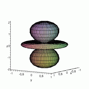
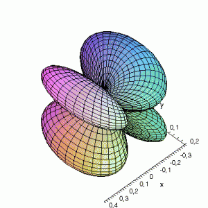
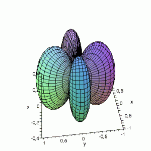
3D Maple-images of the d-orbitals S02(θ,φ), S12(θ,φ) en S22(θ,φ). Note that the spherical coordinates (θ and φ) used by Maple are reversed compared to the definitions used in Griffiths’ Introduction to Quantum Mechanics (the latter being the more standard definition in physics and mathematics courses).
S02(θ,φ)
> plot3d(abs(3*cos(phi)*cos(phi)-1),theta=0..Pi,phi=0..2*Pi,
grid=[60,60],coords=spherical,axes=frame,labels=[x,y,z]);
S12(θ,φ)
> plot3d(abs(sin(phi)*cos(phi)*cos(theta)),theta=0..2*Pi,phi=0..Pi,
grid=[60,60],coords=spherical,axes=frame,labels=[x,y,z]);
S22(θ,φ)
> plot3d(abs(sin(phi)*sin(phi)*cos(2*theta)),theta=0..2*Pi,phi=0..Pi,
grid=[60,60],coords=spherical,axes=frame,labels=[x,y,z]);
Effect of exchanging θ and φ
Maple assumes the first angle given is the angle in the xy-plane; the second angle is with regard to the z-axis. This makes that you have to be very careful when giving Maple the θ and φ angles, and make sure that their definitions are the same. If the definitions
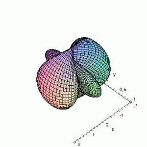
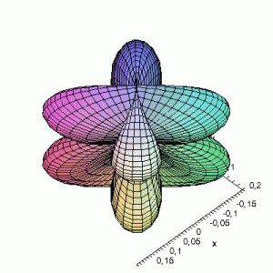
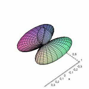
are reversed: I.e. if we use the variable θ as the variable φ and vice versa, the resulting plots become something quite different. This goes for all available plotting programs (Maple, gnuplot…); make sure you certain that what you think you enter is also what the program thinks you have entered. If not you could end up with surprising results. The same images as above, but now with θ and φ exchanged:
are reversed: I.e. if we use the variable θ as the variable φ and vice versa, the resulting plots become something quite different. This goes for all available plotting programs (Maple, gnuplot…); make sure you certain that what you think you enter is also what the program thinks you have entered. If not you could end up with surprising results. The same images as above, but now with θ and φ exchanged:
