After the exam period in weeks nine and ten, the eleventh and twelfth week of the academic year bring the second quarter of our materiomics program at UHasselt for the first master students. Although I’m not coordinating any courses in this quarter, I do have some teaching duties, including being involved in two of the hands-on projects.
As in the past 10 weeks, the bachelor students in chemistry had lectures for the courses introduction to quantum chemistry and quantum and computational chemistry. For the second bachelor this meant they finally came into contact with the H atom, the first and only system that can be exactly solved using pen and paper quantum chemistry (anything beyond can only be solved given additional approximations.) During the exercise class we investigated the concept of aromatic stabilization in more detail in addition to the usual exercises with simple Schrödinger equations and wave functions. For the third bachelor, their travel into the world of computational chemistry continued, introducing post-Hartree-Fock methods with also include the missing correlation energy. This is the failure of Hartree-Fock theory, making it a nice framework, but of little practical use for any but the most trivial molecules (e.g. H2 for example already being out of scope). We also started looking into molecular systems, starting with simple diatomic molecules like H2+.
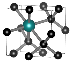
SnV split vacancy defect in diamond.
In the master materiomics, the course Machine learning and artificial intelligence in modern materials science hosted a guest lecture on Large Language Models, and their use in materials research as well as an exercise session during which the overarching ML study of the QM9 dataset was extended. During the course on Density Functional Theory there was a second lab, this time on conceptual DFT. For the first master students, the hands-on project kept them busy. One group combining AI and experiments, and a second group combining DFT modeling of SnV0 defects in diamond with their actual lab growth. It was interesting to see the enthusiasm of the students. With only some mild debugging, I was able to get them up and running relatively smoothly on the HPC. I am also truly grateful to our experimental colleagues of the diamond growth group, who bravely set up these experiments and having backup plans for the backup plans.
At the end of week 12, we added another 12h of classes, ~1h of video lecture, ~2h of HPC support for the handson project and 6h of guest lectures, putting our semester total at 118h of live lectures. Upwards and onward to weeks 13 & 14.


 During the last year,