When running programs on HPC infrastructure, one of the first questions to ask yourself is: “How well does this program scale?“
In applications for HPC resources, this question plays a central role, often with the additional remark: “But for your specific system!“. For some software packages this is an important remark, for other packages this remark has little relevance, as the package performs similarly for all input (or for given classes of input). The VASP package is one of the latter. For my current resource application at the Flemish TIER-1 I set out to do a more extensive scaling test of the VASP package. This is for 2 reasons. The first being the fact that I will be using a newer version of VASP: vasp 5.4.1 (I am currently using my own multiply patched version 5.3.3.). The second being the fact that I will be using a brand new TIER-1 machine (second Flemish TIER-1, as our beloved muk retired the end of 2016).
Why should I put in the effort to get access to resources on such a TIER-1 supercomputer? Because such machines are the life blood of the computational materials scientist. They are their sidekick in the quest for understanding of materials. Over the past 4 years, I was granted (and used) 20900 node-days of calculation time (i.e. over 8 Million hours of CPU time, or 916 years of calculation time) on the first TIER-1 machine.
Now back to the topic. How well does VASP 5.4.1 behave? That depends on the system at hand, and how good you choose the parallelization settings.
1. Parallelization in VASP
VASP provides several parameters which allow for straightforward parallelization of the simulation:
- NPAR : This parameter can be set to parallelize over the electronic bands. As a consequence, the number of bands included in a calculation by VASP will be a multiple of NPAR. (Note : Hybrid calculations are an exception as they require NPAR to be set to the number of cores used per k-point.)
- NCORE : The NCORE parameter is related to NPAR via NCORE=#cores/NPAR, so only one of these can be set.
- KPAR : This parameter can be set to parallelize over the set of irreducible k-points used to integrate over the first Brillouin zone. KPAR should therefore best be a divisor of the number of irreducible k-points.
- LPLANE : This boolean parameter allows one to switch on parallelization over plane waves. In general this will give rise to a small but consistent speedup (observed in previous scaling tests). As such we have chosen to set this parameter = .TRUE. for all calculations.
- NSIM : Sets up a blocked mode for the RMM-DIIS algorithm. (cf. manual, and further tests by Peter Larsson). As our tests do not involve the RMM-DIIS algorithm, this parameter was not set.
In addition, one needs to keep the architecture of the HPC-system in mind as well: NPAR, KPAR and their product should be divisors of the number of nodes (and cores) used.
2. Results
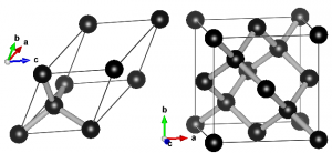
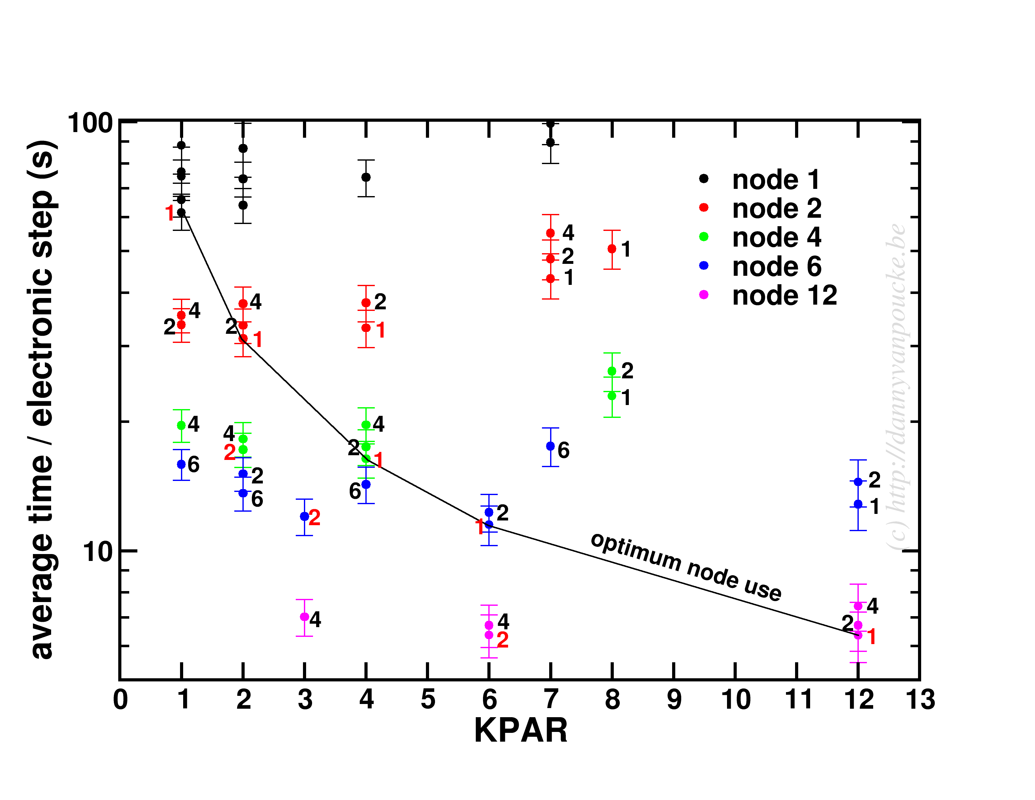
Both NPAR and KPAR parameters can be set simultaneously and will have a serious influence on the speed of your calculations. However, not all possible combinations give the same speedup. Even worse, not all combinations are beneficial with regard to speed. This is best seen for a small 2 atom diamond primitive cell.
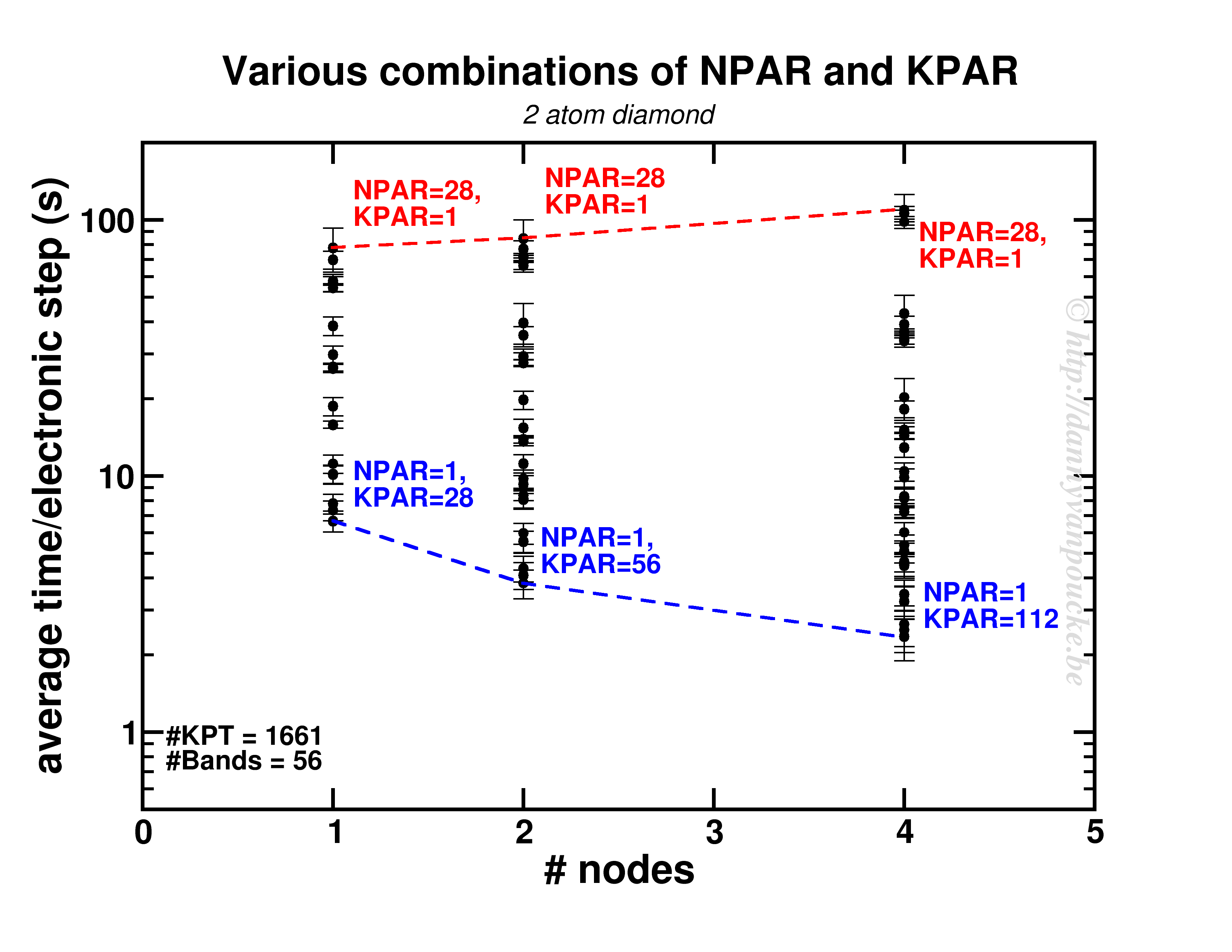
Timing results for various combinations of the NPAR and KPAR parameters for a 2 atom primitive unit cell of diamond.
Two things are clear. First of all, switching on a parallelization parameter does not necessarily mean the calculation will speed up. In some case it may actually slow you down. Secondly, the best and worst performance is consistently obtained using the same settings. Best: KPAR = maximal, and NPAR = 1, worst: KPAR = 1 and NPAR = maximal.
This small system shows us what you can expect for systems with a lot of k-points and very few electronic bands ( actually, any real calculation on this system would only require 8 electronic bands, not 56 as was used here to be able to asses the performance of the NPAR parameter.)
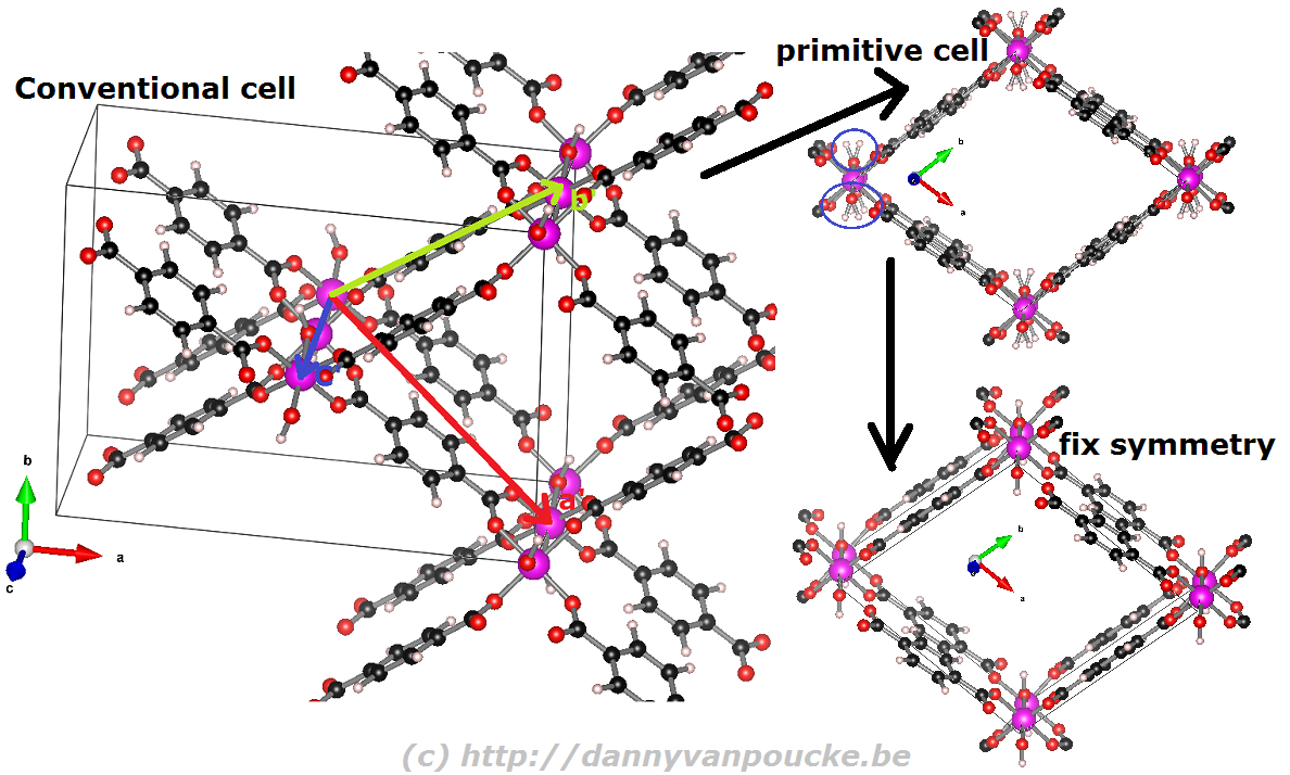
In a medium sized system (20-100 atoms), the situation will be different. There, the number of k-points will be small (5-50) while the natural number of electronic bands will be large (>100). As a test-case I looked at my favorite Metal-Organic Framework: MIL-47(V).
Timing results for several NPAR/KPAR combinations for the MIL-47(V) system.
This system has only 12 k-points to parallelize over, and 224 electronic bands. The spread per number of nodes is more limited than for the small system. In contrast, the general trend remains the same: KPAR=high, NPAR=low, with an optimum performance when KPAR=#nodes. Going beyond standard DFT, using hybrid functionals, also retains the same picture, although in some cases about 10% performance can be gained when using one half node per k-point. Unfortunatly, as we have very few k-points to start from, this will only be an advantage if the limiting factor is the number of nodes available.
An interesting behaviour is seen when one keeps the k-points/#nodes ratio constant:
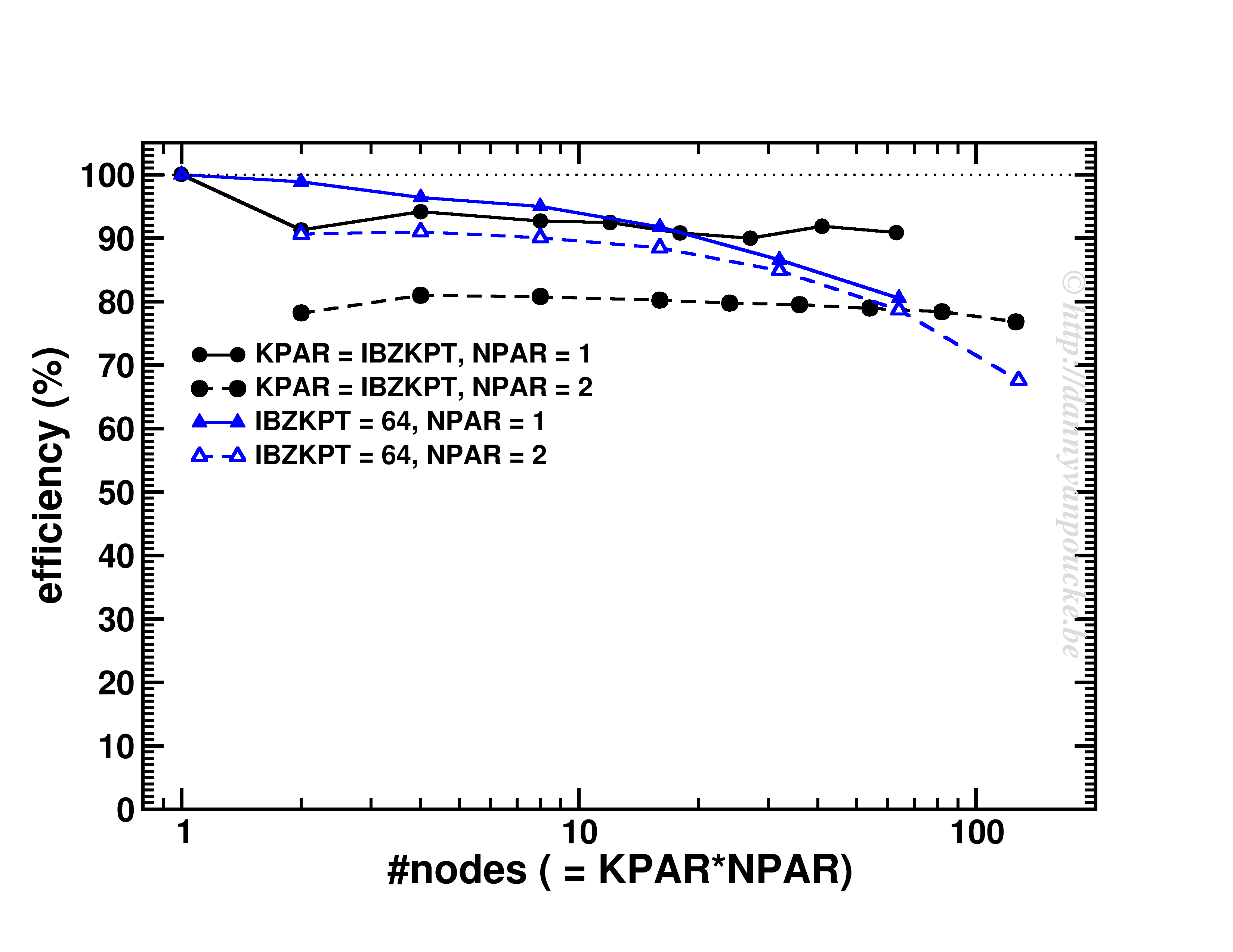
Scaling behavior for either a constant number of k-points (for dense k-point grid in medium sized system) or constant k-point/#nodes ratio.
As you can see, VASP performs really well up to KPAR=#k-points (>80% efficiency). More interestingly, if the k-point/#node ratio is kept constant, the efficiency (now calculated as T1/(T2*NPAR) with T1 timing for a single node, and T2 for multiple nodes) is roughly constant. I.e. if you know the walltime for a 2-k-point/2-nodes job, you can use/expect the same for the same system but now considering 20-k-points/20-nodes (think Density of States and Band-structure calculations, or just change of #k-points due to symmetry reduction or change in k-point grid.) 😆
3. Conclusions and Guidelines
If one thing is clear from the current set of tests, it is the fact that good scaling is possible. How it is attained, however, depends greatly on the system at hand. More importantly, making a poor choice of parallelization settings can be very detrimental to the obtained speed-up and efficiency. Unfortunately when performing calculations on an HPC system, one has externally imposed limitations to work with:
- Memory available per core
- Number of cores per node[1]
- Size of your system: #atoms, #k-points, & #bands
Here are some guidelines (some open doors as well):
- Wherever possible k-point parallelization should be driven to a maximum (KPAR as large as possible). The limiting factor here is the actual number of k-points and the amount of memory available. The latter due to the fact that a higher value of KPAR leads to a higher memory requirement.[2]
- Use the Γ-version of VASP for Γ-point only calculations. It reduces memory usage significantly (3.7Gb→ 2.8Gb/core for a 512 atom diamond system) and increases the computational efficiency, sometimes even by a factor of 2.
- NPAR parallelization can be used to reduce the memory load for high KPAR calculations, but increasing KPAR will always outperform the same increase of NPAR.
- In case only NPAR parallelization is available, due to too few k-points, and working with large systems, NPAR parallelization is your last resort, and will perform reasonably well, up to a point.
- Electronic steps show very consistent timing, so scaling tests can be performed with only a 5-10 electronic steps, with standard deviations comparable in absolute size for PBE and HSE06.
In short:
K-point parallelism will save you, wherever possible !
[1] 28 is a lousy number in that regard as its prime-decomposition is 2x2x7, leaving little overlap with prime-decompositions of the number of k-points, which more often than you wish end up being prime numbers themselves 😥
[2] The small system’s memory requirements varied from 0.15 to 1.09 Gb/core for the different combinations.