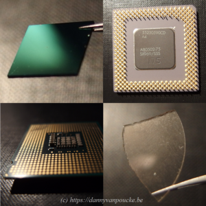
Diamond and CPU’s, now still separated, but how much longer will this remain the case?
Top left: Thin film N-doped diamond on Si (courtesy of Sankaran Kamatchi). Top right: Very old Pentium 1 CPU from 1993 (100MHz), with µm architecture. Bottom left: more recent intel core CPU (3GHz) of 2006 with nm scale architecture. Bottom right: Piece of single crystal diamond. A possible alternative for silicon, with 20x higher thermal conductivity, and 7x higher mobility of charge carriers.
Can you pitch your research in 3 minutes, this is the concept behind “wetenschap uitgedokterd/science figured out“. A challenge I accepted after the fun I had at the science-battle. If I can explain my work to a public of 6 to 12 year-olds, explaining it to adults should be possible as well. However, 3 minutes is very short (although some may consider this long in the current bitesize world), especially if you have to explain something far from day-to-day life and can not assume any scientific background.
Where to start? Capture the imagination: “Imagine a world where you are a god.”
Link back to the real world. “All modern-day high-tech toys are more and more influenced by the atomic scale details.” Over the last decade, I have seen the nano-scale progress slowly but steadily into the realm of real-life materials research. This almost invisible trend will have a huge impact on materials science in the coming decade, because more and more we will see empirical laws breaking down, and it will become harder and harder to fit trends of materials using a classical mindset, something which has worked marvelously for materials science during the last few centuries. Modern and future materials design (be it solar cells, batteries, CPU’s or even medicine) will have to rely on quantum mechanical intuition and hence quantum mechanical simulations. (Although there is still much denial in that regard.)
Is there a problem to be solved? Yes indeed: “We do not have quantum mechanical intuition by nature, and manipulating atoms is extremely hard in practice and for practical purposes.” Although popular science magazines every so often boast pictures of atomic scale manipulation of atoms and the quantum regime, this makes it far from easy and common inside and outside the university lab. It is amazing how hard these things tend to get (ask your local experimental materials research PhD) and the required blood, sweat and tears are generally not represented in the glory-parade of a scientific publication.
Can you solve this? Euhm…yes…at least to some extend. “Computational materials research can provide the quantum mechanical intuition we human beings lack, and gives us access to atomic scale manipulation of a material.” Although computational materials science is seen by experimentalists as theory, and by theoreticians as experiments, it is neither and both. Computational materials science combines the rigor and control of theory, with access to real-life systems of experiments. It, unfortunately also suffers the limitations of both: as the system is still idealized (but to much lesser extend than in theoretical work) and control is not absolute (you have to follow where the algorithms take you, just as an experimentalist has to follow where the reaction takes him/her). But, if these strengths and weaknesses are balanced wisely (requires quite a few years of experience) an expert will gain fundamental insights in experiments.

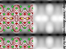
Animation representing the buildup of a diamond surface in computational work.
As a computational materials scientist, you build a real-life system, atom by atom, such that you know exactly where everything is located, and then calculate its properties based on the rules of quantum mechanics, for example. In this sense you have absolute control as in theory. This comes at a cost (conservation of misery 🙂 ); where nature itself makes sure the structure is the “correct one” in experiments, you have to find it yourself in computational work. So you generally end up calculating many possible structural combinations of your atoms to first find out which is the one most probable to represent nature.
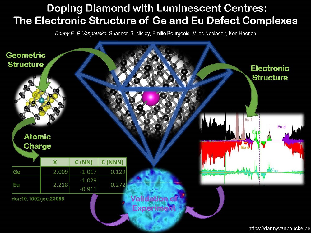
So what am I actually doing? “I am using atomic scale quantum mechanical computations to investigate the materials my experimental colleagues are studying, going from oxides to defects in diamond.” I know this is vague, but unfortunately, the actual work is technical. Much effort goes into getting the calculations to run in the direction you want them to proceed (This is the experimental side of computational materials science.). The actual goal varies from project to project. Sometimes, we want to find out which material is most stable, and which material is most likely to diffuse into the other, while at other times we want to understand the electronic structure, to test if a defect is really luminescent, this to trace the source of the experimentally observed luminescence. Or if you want to make it more complex, even find out which elements would make diamond grow faster.
Starting from this, I succeeded in creating a 3-minute pitch of my research for Science Figured out. The pitch can be seen here (in Dutch, with English subtitles that can be switched on through the cogwheel in the bottom right corner).
Some external links:
 About 10 years ago, at the end of 2007 and beginning of 2008, the 5 Flemish universities founded the Flemish Supercomputer Center (