Tag: science communication

Roots of Science

Today VLIR (Flemish Inter-university Council) and the Young Academy had a conference on the future of fundamental research in Flanders: Roots of Science. We live in a world where we rely on science more and more to resolve our problems (think climate change, disease control, energy generation, …). In our bizarre world of alternative facts and fake news, science can be utterly ignored in one sentence and proposed as a magical solution in the next.

Although I am happy with the faith some have in the possibilities of science, it is important to remember that it is not magic. This has a very important consequence:

Things do not happen simply because you want them to happen.


Many important breakthroughs in science are what one would call serendipity (e.g., the discovery of penicillin by Fleming, development of the WWW as a side-effect of researchers wanting to share their data

at CERN in 1991,…) . In Flanders the Royal Flemish Academy and the Young Academy have written a Standpoint (an evidence-based advisory text)

discussing the need for more researcher-driven research in contrast to agenda-driven research, as they believe this is a conditio sine qua non for a healthy scientific future.

Where government-driven research focuses on resolving questions from society, researcher-driven research allows the researcher to follow his or her personal interest. This not with the primal aim of having short-te

rm return of investment, but with the aim of providing the fundamental knowledge and expertise which some day may be needed for the former. In researcher-driver research, the journey is the goal as this is where scientific progress is made by finding solutions for problems not imagined before.

Do we have to pay for this with our tax-payers money? I think we do. No-one imagined optical drives (CD, DVD, blue-ray) to become a billion euro industry while the laser was being developed in a lab. Who would have thought the transistor would play such an important role in our every-day life? And what about the first computer? Thomas Watson, President of IBM, has allegedly said in 1943: “I think there is a world market for maybe 5 computers.” And, yet, now many of us have more than 5 computers at home (including tables, smartphones,…)! The researchers working on these “inventions” did not do this with your Blue-ray player or smartphone in mind. These high impact applications are “merely” side-products of their fundamental scientific research. No-one at the time could predict this, so why should we be able to do this today? In this sense, you should see funding of fundamental research as a long term investment. Tax-money is being invested in our future, and the future of children and grandchildren. Although we do not know what will be the outcome, we know from the past that it will have an impact on our lives.

Its difficult to make predictions, especially about the future.

Let us therefor support more researcher-driven research.


In addition to the Standpoint, there is also a very nice video explaining the situation (with subtitles in English or Dutch, use the cogwheel to select your preference).

Newsflash: Materials of the Future

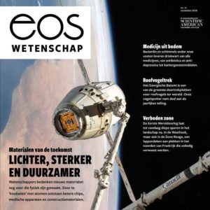
This summer, I had the pleasure of being interviewed by Kim Verhaeghe, a journalist of the EOS magazine, on the topic of “materials of the future“. Materials which are currently being investigated in the lab and which in the near or distant future may have an enormous impact on our lives. While brushing up on my materials (since materials with length scales of importance beyond 1 nm are generally outside my world of accessibility), I discovered that to cover this field you would need at least an entire book just to list the “materials of the future”. Many materials deserve to be called materials of the future, because of their potential. Also depending on your background other materials may get your primary attention.

In the resulting article, Kim Verhaeghe succeeded in presenting a nice selection, and I am very happy I could contribute to the story. Introducing “the computational materials scientist” making use of supercomputers such as BrENIAC, but also new materials such as Metal-Organic Frameworks (MOF) and shedding some light on “old” materials such as diamond, graphene and carbon nanotubes.

Dangerous travel physics

Tossing coins into a fountain brings luck, tossing them of a building causes death and destruction?


We have probably all done it at one point when traveling: thrown a coin into a wishing well or a fountain. There are numerous wishing wells with legends describing how the deity living in the well will bring good fortune in return for this gift. The myths and legends often originate from Celtic, German or Nordic traditions.

In case of the Trevi fountain, there is the belief that if you throw a coin over your left shoulder using your right hand, you will return to Rome…someday. As this fountain and legend are iconic parts of our western movie history, many, many coins get tossed into it (more than 1 Million € worth each year, which is collected an donated to charity).

In addition to these holiday legends, there also exist more recent “coin-myths”: Death by falling penny. These myths are always linked to tall buildings, and claim that a penny dropped from the top of such a building could kill someone if they hit him.

Traveling with Newton

In both kinds of coin legends, the trajectory of the coin can be predicted quite well using Newton’s Laws. Their speed is low compared to the speed of light, and the coins are sufficiently large to keep the world of quantum mechanics hidden from sight.

The second Law of Newton states that the speed of an object changes if there is a force acting on it. Here on earth, gravity is a major player (especially for Physics exercises). In case of a coin tossed into a fountain, gravity will cause the coin to follow a roughly parabolic path before disappearing into the water. The speed at which the coin will hit the water will be comparable to the speed with which it was thrown…at least if there isn’t to much of a difference in height between the surface of the water and the hand of the one throwing the coin.

But, what if this difference is large? Such as in case of the penny being dropped from a tall building. In such a case, the initial velocity is zero, and the penny is accelerated toward the ground by gravity. Using the equations of motion for a uniform accelerated system, we can calculate easily the speed at which the coin hits the ground:

x = x0 + v0*t + ½ * g * t²

v=v0+g*t

If we drop a penny from the 3rd floor of the Eiffel Tower (x0=276.13m, x=0m, v0=0 m/s, g=-9.81m/s²) then the first equation teaches us that after 7.5 seconds, the penny will hit the ground with a final speed (second equation) of -73.6 m/s (or -265 km/h)*. With such a velocity, the penny definitely will leave an impression. More interestingly, we will get the exact same result for a pea (cooked or frozen), a bowling ball, a piano or an anvil…but also a feather. At this point, your intuition must be screaming at you that you are missing something important.

All models are wrong…but they can be very useful

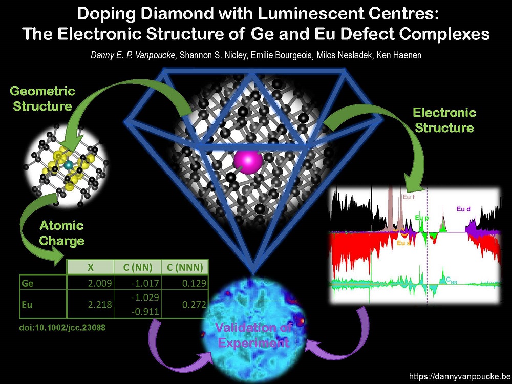
The power of models in physics, originates from keeping only the most important and relevant aspects. Such approximations provide a simplified picture and allow us to understand the driving forces behind nature itself. However, in this context, models in physics are approximations of reality, and thus by definition wrong, in the sense that they do not provide an “exact” representation of reality. This is also true for Newton’s Laws, and our application above. With these simple rules, it is possible to describe the motion of the planets as well as a coin tossed into the Trevi fountain.

So what’s the difference between the coin tossed into a fountain and planetary motion on the one hand, and our assorted objects being dropped from the Eiffel Tower on the other hand?

Friction as it presents itself in aerodynamic drag!

Aerodynamic drag gives rise to a force in the direction opposite to the movement, and it is defined as:

FD= ½ *Rho*v²*CD*A

This force depends on the density Rho of the medium (hence water gives a larger drag than air), the velocity and surface area A in the direction of movement of the object, and CD the drag coefficient, which depends on the shape of the object.

If we take a look at the planets and the coin tosses, we notice that, due to the absence of air between the planets, no aerodynamic drag needs to be considered for planetary motion. In case of a coin being tossed into the Trevi fountain, there is aerodynamic drag, however, the speeds are very low as well as the distance traversed. As such the effect of aerodynamic drag will be rather small, if not negligible. In case of objects being dropped from a tall building, the aerodynamic drag will not be negligible, and it will be the factors CD and A which will make sure the anvil arrives at the ground level before the feather.

Because this force also depends on the velocity, you can no longer make direct use of the first two equations to calculate the time of impact and velocity at each point of the path. You will need a numerical approach for this (which is also the reason this is not (regularly) taught in introductory physics classes at high school). However, using excel, you can get a long way in creating a numerical solution for this problem.[Excel example]

As we know the density of air is about 1.2kg/m³, CD for a thin cylinder (think coin) is 1.17, the radius of a penny is 9.5 mm and its mass is 2.5g, then we can find the terminal velocity of the penny to be 11.1 m/s (40 km/h). The penny will land on the ground after about 25.6 seconds. This is quite a bit slower than what we found before, and also quite a bit more safe. The penny will reach its terminal velocity after having fallen about 60 m, which means that dropping a penny from taller buildings (the Atomium [102 m], the Eiffel Tower [276.13 m, 3rd floor, 324 m top], the Empire State Building [381 m] or even the Burj Khalifa [829.8 m]) will have no impact on the velocity it will have when hitting the ground: 40km/h.

This is a collision you will most probably survive, but which will definitely leave a small bruise on impact.


*The minus sign indicates the coin is falling downward.

Book chapter: Computational Chemistry Experiment Possibilities

Authors: Bartłomiej M. Szyja and Danny Vanpoucke
Book: Zeolites and Metal-Organic Frameworks, (2018)
Chapter Ch 9, p 235-264
Title Computational Chemistry Experiment Possibilities
ISBN: 978-94-629-8556-8
export: bibtex
pdf: <Amsterdam University Press>
<Open Access>


Zeolites and Metal-Organic Frameworks (the hard-copy)

Abstract

Thanks to a rapid increase in the computational power of modern CPUs, computational methods have become a standard tool for the investigation of physico-chemical phenomena in many areas of chemistry and technology. The area of porous frameworks, such as zeolites, metal-organic frameworks (MOFs) and covalent-organic frameworks (COFs), is not different. Computer simulations make it possible, not only to verify the results of the experiments, but even to predict previously inexistent materials that will present the desired experimental properties. Furthermore, computational research of materials provides the tools necessary to obtain fundamental insight into details that are often not accessible to physical experiments.

The methodology used in these simulations is quite specific because of the special character of the materials themselves. However, within the field of porous frameworks, density functional theory (DFT) and force fields (FF)
are the main actors. These methods form the basis of most computational studies, since they allow the evaluation of the potential energy surface (PES) of the system.

Related:

Newsflash: here

Building bridges towards experiments.

Quantum Holy Grail: The Ground-State

Quantum mechanical calculations provide a powerful tool to investigate the world around us. Unfortunately it is also a computationally very expensive tool to use, which puts a boundary on what is possible in terms of computational materials research. For example, when investigating a solid at the quantum mechanical level, you are limited in the number of atoms that you can consider. Even with a powerful supercomputer at hand, a hundred to a thousand atoms are currently accessible for “routine” investigations. The computational cost also limits the number of configurations/combinations you can calculate.

However, in the end— and often with some blood sweat and tears—these calculations do provide you the ground-state structure and energy of your system. From this point forward you can continue characterizing its properties, life is beautiful and happy times are just beyond the horizon. At this horizon your experimental colleague awaits you. And he/she tells you:

Sorry, I don’t find that structure in my sample.

After recovering from the initial shock, you soon realize that in (materials science) experiments one seldom encounters a sample in “the ground-state”. Experiments are performed at temperatures above 0K and pressures above 0 Pa (even in vacuum :p ). Furthermore, synthesis methods often involve elevated temperatures, increased pressure, mechanical forces, chemical reactions,… which give rise to meta-stable configurations. In such an environment, your nicely deduced ground-state may be an exception to the rule. It is only one point within the phase-space of the possible.

So how can you deal with this? You somehow need to sample the phase-space available to the experiment.

Sampling Phase-Space for Ball-milling synthesis.

For a few years now, I have a very fruitful collaboration with Prof. Rounaghi. His interest goes toward the cheap fabrication of metal-nitrides. Our first collaboration focused on AlN, while later work included Ti, V and Cr-nitrides. Although this initial work had a strong focus on simple corroboration through the energies calculated at the quantum mechanical level, the collaboration also allowed me to look at my data in a different way. I wanted to “simulate” the reactions of ball-milling experiments more closely.

Due to the size-limitations of quantum mechanical calculations I played with the following idea:

  • Assume there exists a general master reaction which describes what happens during ball-milling.

X Al + Y Melamine → x1 Al + x2 Melamine + x3 AlN + …

where all the xi represent the fractions of the reaction products present.

  • With the boundary condition that the number of particles needs to be conserved, you end up with a large set of (x1,x2,x3,…) configurations which each have a certain energy. This energy is calculated using the quantum mechanical energies of each product. The configuration with the lowest energy is the ground state configuration. However, investigating the entire accessible phase-space showed that the energies of the other possible configurations are generally not that much higher.
  • What if we used the energy available due to ball-milling in the same fashion as we use kBT? And sample the phase-space using Boltzmann statistics.
  • The resulting Boltzmann distribution of the configurations available in the phase-space can then be used to calculate the mass/atomic fraction of each of the products and allow us to represent an experimental sample as a collection of small units with slightly different configurations, weighted according to their Boltzmann distribution.

This setup allowed me to see the evolution in end-products as function of the initial ratio in case of AlN, and in our current project to indicate the preferred Iron-nitride present.

Grid-sampling vs Monte-Carlo-sampling

Whereas the AlN system was relatively easy to investigate—the phase space was only 3 dimensional— the recent iron based system ended up being 4 dimensional when considering only host materials, and 10 dimensional when including defects. For a small 3-4D phase-space, it is possible to create an equally spaced grid and get converged results using a few million to a billion grid-points. For a 10D phase-space this is no longer possible. As you can no longer keep all data-points (easily) in storage during your calculation (imagine 1 Billion points, requiring you to store 11 double precision floats or about 82Gb) you need a method that does not rely on large arrays of data. For our Boltzmann statistics this gives us a bit of a pickle, as we need to have the global minimum of our phase space. A grid is too course to find it, while a simple Monte-Carlo just keeps hopping around.

Using Metropolis’s improvement of the Monte-Carlo approach was an interesting exercise, as it clearly shows the beauty and simplicity of the approach. This becomes even more awesome the moment you imagine the resources available in those days. I noted 82Gb being a lot, but I do have access to machines with those resources; its just not available on my laptop. In those days MANIAC supercomputers had less than 100 kilobyte of memory.

Although I theoretically no longer need the minimum energy configuration, having access to that information is rather useful. Therefore, I first search the phase-space for this minimum. This is rather tricky using Metropolis Monte Carlo (of course better techniques exist, but I wanted to be a bit lazy), and I found that in the limit of T→0 the algorithm will move toward the minimum. This, however, may require nearly 100 million steps of which >99.9% are rejected. As it only takes about 20 second on a modern laptop…this isn’t a big issue.

Finding a minimum using Metropolis Monte Carlo.

Finding a minimum using Metropolis Monte Carlo.

Next, a similar Metropolis Monte Carlo algorithm can be used to sample the entire phase space. Using 109 sample points was already sufficient to have a nicely converged sampling of the phase space for the problem at hand. Running the calculation for 20 different “ball-milling” energies took less than 2 hours, which is insignificant, when compared to the resources required to calculate the quantum mechanical ground state energies (several years). The figure below shows the distribution of the mass fraction of one of the reaction products as well as the distribution of the energies of the sampled configurations.

Metropolis Monte Carlo distribution of mass fraction and configuration energies for 3 sets of sample points.

Metropolis Monte Carlo distribution of mass fraction and configuration energies for 3 sets of sample points.

This clearly shows us how unique and small the quantum mechanical ground state configuration and its contribution is compared to the remainder of the phase space. So of course the ground state is not found in the experimental sample but that doesn’t mean the calculations are wrong either. Both are right, they just look at reality from a different perspective. The gap between the two can luckily be bridged, if one looks at both sides of the story. 


Science Figured out

Diamond and CPU's, now still separated, but how much longer will this remain the case? Top left: Thin film N-doped diamond on Si (courtesy of Sankaran Kamatchi). Top right: Very old Pentium 1 CPU from 1993 (100MHz), with µm architecture. Bottom left: more recent intel core CPU (3GHz) of 2006 with nm scale architecture. Bottom right: Piece of single crystal diamond. A possible alternative for silicon, with 20x higher thermal conductivity, and 7x higher mobility of charge carriers.

Diamond and CPU’s, now still separated, but how much longer will this remain the case?
Top left: Thin film N-doped diamond on Si (courtesy of Sankaran Kamatchi). Top right: Very old Pentium 1 CPU from 1993 (100MHz), with µm architecture. Bottom left: more recent intel core CPU (3GHz) of 2006 with nm scale architecture. Bottom right: Piece of single crystal diamond. A possible alternative for silicon, with 20x higher thermal conductivity, and 7x higher mobility of charge carriers.

Can you pitch your research in 3 minutes, this is the concept behind “wetenschap uitgedokterd/science figured out“. A challenge I accepted after the fun I had at the science-battle. If I can explain my work to a public of 6 to 12 year-olds, explaining it to adults should be possible as well. However, 3 minutes is very short (although some may consider this long in the current bitesize world), especially if you have to explain something far from day-to-day life and can not assume any scientific background.

Where to start? Capture the imagination: “Imagine a world where you are a god.

Link back to the real world. “All modern-day high-tech toys are more and more influenced by the atomic scale details.” Over the last decade, I have seen the nano-scale progress slowly but steadily into the realm of real-life materials research. This almost invisible trend will have a huge impact on materials science in the coming decade, because more and more we will see empirical laws breaking down, and it will become harder and harder to fit trends of materials using a classical mindset, something which has worked marvelously for materials science during the last few centuries. Modern and future materials design (be it solar cells, batteries, CPU’s or even medicine) will have to rely on quantum mechanical intuition and hence quantum mechanical simulations. (Although there is still much denial in that regard.)

Is there a problem to be solved? Yes indeed: “We do not have quantum mechanical intuition by nature, and manipulating atoms is extremely hard in practice and for practical purposes.” Although popular science magazines every so often boast pictures of atomic scale manipulation of atoms and the quantum regime, this makes it far from easy and common inside and outside the university lab. It is amazing how hard these things tend to get (ask your local experimental materials research PhD) and the required blood, sweat and tears are generally not represented in the glory-parade of a scientific publication.

Can you solve this? Euhm…yes…at least to some extend. “Computational materials research can provide the quantum mechanical intuition we human beings lack, and gives us access to atomic scale manipulation of a material.” Although computational materials science is seen by experimentalists as theory, and by theoreticians as experiments, it is neither and both. Computational materials science combines the rigor and control of theory, with access to real-life systems of experiments. It, unfortunately also suffers the limitations of both: as the system is still idealized (but to much lesser extend than in theoretical work) and control is not absolute (you have to follow where the algorithms take you, just as an experimentalist has to follow where the reaction takes him/her). But, if these strengths and weaknesses are balanced wisely (requires quite a few years of experience) an expert will gain fundamental insights in experiments.

Animation representing the buildup of a diamond surface in computational work.

Animation representing the buildup of a diamond surface in computational work.

As a computational materials scientist, you build a real-life system, atom by atom, such that you know exactly where everything is located, and then calculate its properties based on the rules of quantum mechanics, for example. In this sense you have absolute control as in theory. This comes at a cost (conservation of misery 🙂 ); where nature itself makes sure the structure is the “correct one” in experiments, you have to find it yourself in computational work. So you generally end up calculating many possible structural combinations of your atoms to first find out which is the one most probable to represent nature.

So what am I actually doing?I am using atomic scale quantum mechanical computations to investigate the materials my experimental colleagues are studying, going from oxides to defects in diamond.” I know this is vague, but unfortunately, the actual work is technical. Much effort goes into getting the calculations to run in the direction you want them to proceed (This is the experimental side of computational materials science.). The actual goal varies from project to project. Sometimes, we want to find out which material is most stable, and which material is most likely to diffuse into the other, while at other times we want to understand the electronic structure, to test if a defect is really luminescent, this to trace the source of the experimentally observed luminescence. Or if you want to make it more complex, even find out which elements would make diamond grow faster.

Starting from this, I succeeded in creating a 3-minute pitch of my research for Science Figured out. The pitch can be seen here (in Dutch, with English subtitles that can be switched on through the cogwheel in the bottom right corner).

Some external links:


VSC User Day 2018

Today, I am attending the 4th VSC User Day at the “Paleis de Academiën” in Brussels. Flemish researchers for whom the lifeblood of their research flows through the chips of a supercomputer are gathered here to discuss their experiences and present their research.

Some History

About 10 years ago, at the end of 2007 and beginning of 2008, the 5 Flemish universities founded the Flemish Supercomputer Center (VSC). A virtual organisation with one central goal:  Combine their strengths and know-how with regard to High Performance Compute (HPC) centers to make sure they were competitive with comparable HPC centers elsewhere.

By installing a super-fast network between the various university compute centers, each Flemish researcher has nowadays access to state-of-the-art computer infrastructure, independent of his or her physical location. A researcher at the University of Hasselt, like myself, can easily run calculations on the supercomputers installed at the university of Ghent or Leuven. In October 2012 the existing university supercomputers, so-called Tier-2 supercomputers, are joined by the first Flemish Tier-1 supercomputer, which was housed at the brand new data-centre of Ghent University. This machine is significantly larger than the existing Tier-2 machines, and allows Belgium to become the 25th member of the PRACE network, a European network which provides computational researchers access to the best and largest computer facilities in Europe. The fast development of computational research in Flanders and the explosive growth in the number of computational researchers, combined with the first shared Flemish supercomputer (in contrast to the university TIER-2 supercomputers, which some still consider private property rather than part of VSC) show the impact of the virtual organisation that is the VSC. As a result, on January 16th 2014, the first VSC User Day is organised, bringing together HPC users from all 5 universities  and industry. Here the users share their experiences and discuss possible improvements and changes. Since then, the first Tier-1 supercomputer has been decommissioned and replaced by a brand new Tier-1 machine, this time located at the KU Leuven. Furthermore, the Flemish government has put 30M€ aside for super-computing in Flanders, making sure that also in the future Flemish computational research stays competitive. The future of computational research in Flanders looks bright.

Today is User Day 2018

During the 4th VSC User Day, researchers of all 5 Flemish universities will be presenting the work they are performing on the supercomputers of the VSC network. The range of topics is very broad: from first principles materials modelling to chip design, climate modelling and space weather. In addition there will also be several workshops, introducing new users to the VSC and teaching advanced users the finer details of GPU-code and code optimization and parallelization. This later aspect is hugely important during the use of supercomputers in an academic context. Much of the software used is developed or modified by the researchers themselves. And even though this software can present impressive behavior, it doe not speed up automatically if you provide it access to more CPU’s. This is a very non-trivial task the researchers has to take care of, by carefully optimizing and parallelizing his or her code.

To support the researchers in their work, the VSC came up with ingenious poster-prizes. The three best posters will share 2018 node days of calculation time (about 155 years of calculations on a normal simple computer).

Wish me luck!


Single-slide presentation of my poster @VSC User Day 2018.

Single-slide presentation of my poster @VSC User Day 2018.

Newsflash: Book-chapter on MOFs and Zeolites en route to bookstores near you.

It is almost a year ago that I wrote a book-chapter, together with Bartek Szyja, on MOFs and Zeolites. Coming March 2018, the book will be available through University press. It is interesting to note that in a 13 chapter book, ours was the only chapter dealing with the computational study and simulation of these materials…so there is a lot more that can be done by those who are interested and have the patience to perform these delicate and often difficult but extremely rewarding studies. From my time as a MOF researcher I have learned two important things:

  1. Any kind of interesting/extreme/silly physics you can imagine will be present in some MOFs. In this regard, the current state of the MOF/COF field is still in its infancy as most experimental work focuses on  simple applications such as catalysis and gas storage, for which other materials may be better suited. These porous materials may be theoretically interesting for direct industrial application, but the synthesis cost generally will be a bottleneck. Instead, looking toward the fundamental physics applications: Low dimensional magnetism, low dimensional conduction, spin-filters, multiferroics, electron-phonon interactions, interactions between spin and mechanical properties,…. MOFs are a true playground for the theoretician.
  2. MOFs are very hard to simulate correctly, so be wary of all (published) results that come computationally cheap and easy. Although the unit-cell of any MOF is huge, with regard to standard solid state materials, the electron interactions are also quite long range, so the first Brillouin zone needs very accurate sampling (something often neglected). Also spin-configurations can have a huge influence, especially in systems with a rather flat potential energy surface.

In the book-chapter, we discuss some basic techniques used in the computational study of MOFs, COFs, and Zeolites, which will be of interest to researchers starting in the field. We discuss molecular dynamics and Monte Carlo, as well as Density Functional Theory and all its benefits and limitations.

Open Access version of the book.

Audioslides tryout.

One of the new features provided by Elsevier upon publication is the creation of audioslides. This is a kind of short presentation of the publication by one of the authors. I have been itching to try this since our publication on the neutral C-vancancy was published. The interface is quite intuitive, although the adobe flash tend to have a hard time finding the microphone. However, once it succeeds, things go quite smoothly. The resolution of the slides is a bit low, which is unfortunate (but this is only for the small-scale version, the large-scale version is quite nice as you can see in the link below). Maybe I’ll make a high resolution version video and put it on Youtube, later.

The result is available here (since the embedding doesn’t play nicely with WP).

And a video version can be found here.
 

Functional Molecular Modelling: simulating particles in excel

This semester I had several teaching assignments. I was a TA for the course biophysics for the first bachelor biomedical sciences, supervised two 3rd bachelor students physics during their first steps in the realm of computational materials science, and finally, I was responsible for half the course Functional Molecular Modelling for the first Masters Biomedical students (Bioelectronics and Nanotechnology). In this course, I introduce the the students into the basic concepts of classical molecular modelling (quantum modelling is covered by Prof. Wilfried Langenaeker). It starts with a reiteration of some basic concepts from statistics and moves on to cover the canonical ensemble. Things get more interesting with the introduction into Monte-Carlo(MC) and Molecular Dynamics(MD), where I hope to teach the students the basics needed to perform their own MC and MD simulations. This also touches the heart of what this course should cover. If I hear a title like Functional Molecular Modelling, my thoughts move directly to practical applications, developing and implementing models, and performing simulations. This becomes a bit difficult as none of the students have any programming experience or skills.

Luckily there is excel. As the basic algorithms for MC and MD are actually quite simple, this office package can be (ab)used to allow the students to perform very simple simulations. This even without the use of macro’s or any advanced features. Because Excel can also plot the data present in the cells, you immediately see how properties of the simulated system vary during the simulation, and you get direct update of all graphs every time a simulation is run.

It seems I am not the only one who is using excel for MD simulations. In 1995, Fraser and Woodcock even published a paper detailing the use of excel for performing MD simulations on a system of 100 particles. Their MD is a bit more advanced than the setup I used as it made heavy use of macro’s and needed some features to speed things up as much as possible. With the x486 66MHz computers available at that time, the simulations took of the order of hours. Which was impressive, as they served as an example of how computational speed had improved over the years, and compared to the months of supercomputer resources one of the authors had needed 25 years earlier to perform the same thing for his PhD. Nowadays the same excel simulation should only take minutes, while an actual program in Fortran or C may even execute the same thing in a matter of seconds or less.

For the classes and exercises, I made use of a simple 3-atom toy-model with Lennard-Jones interactions. The resulting simulations remain clear allowing their use for educational purposes. In case of  MC simulations, a nice added bonus is the fact that excel updates all its fields automatically when a cell is modified. As a result, all random numbers are regenerated and a new simulation can be performed by saving the excel-sheet or just modifying a not-used cell.

Monte Carlo in excel. A system of three particles on a line, with one particle fixed at 0. All particles interact through a Lennard-Jones potential. The Monte Carlo simulation shows how the particles move toward their equilibrium position.

Monte Carlo in excel. A system of three particles on a line, with one particle fixed at 0. All particles interact through a Lennard-Jones potential. The Monte Carlo simulation shows how the particles move toward their equilibrium position.

The simplicity of Newton’s equations of motion make it possible to perform simple MD simulations, and already for a three particle system, you can see how unstable the algorithm is. Implementation of the leap-frog algorithm isn’t much more complex and shows incredible the stability of this algorithm. In the plot of the total energy you can even see how the algorithm fights back to retain stability (the spikes may seem large, but the same setup with a straight forward implementation of Newton’s equation of motion quickly moves to energies of the order of 100).

Molecular dynamics in excel. A system of three particles on a line, with one particle fixed at 0. All particles interact through a Lennard-Jones potential. The Molecular dynamics simulation shows how the particles move as time evolves. Their positions are updated using the leap-frog algorithm. The extreme hard nature of the Lennard-Jones potential gives rise to the sharp spikes in the total energy. It is this last aspect which causes the straight forward implementation of Newton's equations of motion to fail.

Molecular dynamics in excel. A system of three particles on a line, with one particle fixed at 0. All particles interact through a Lennard-Jones potential. The Molecular dynamics simulation shows how the particles move as time evolves. Their positions are updated using the leap-frog algorithm. The extreme hard nature of the Lennard-Jones potential gives rise to the sharp spikes in the total energy. It is this last aspect which causes the straight forward implementation of Newton’s equations of motion to fail.