Fabulous Famelab

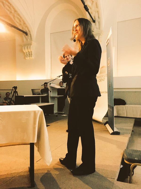
Sylvia convincing the jury at the Famelab heat in Ghent. (thanks to jury member Philippe Smet)

Sylvia convincing the jury at the Famelab heat in Ghent. (Thanks to jury member Philippe Smet)

These days, a scientist is no longer the lone researcher, hiding away in dark rooms and cellars, never coming out, except to ask a servant to mail a letter with his/her newest findings to a like-minded scholar hidden in some other dungeon. Nowadays, we have email to do the latter. In addition, “the scientist” has also had to become the inspiring teacher, the diligent administrator/manager, and the quick salesman/woman pitching his/her ideas for new project-funding. More recently, becoming a rock star was added to this list. (One may start to wonder when she/he should be doing research.)

Since 2005, Famelab, which is part of the Cheltenham Science Festival, has been a platform for young scientist to become such a rock star. In only three minutes, they have to explain a scientific topic of their own choice (and expertise) to the lay public. For this they are allowed only the use of a prop, which they have to be able carry by themselves onto the stage (i.e. no PowerPoint-slides or projected video). Their presentation is then judged by a panel with experience in science communication, focusing on 3 c’s: clarity (the general public should understand what you are going on about), content (it’s not because you present for a general public that you are allowed to cut corners and tell things which aren’t really true) and communication charisma (can you inspire people).

This year, my girlfriend decided to enter the Famelab competition (she’s by far the better communicator of the two of us). During the regional Famelab-heat on April 24th, in my hometown Ghent, she explained in three minutes why we see colours in soap-bubbles (video). The competition during the heat was quite impressive, and of the 25 people who started that day, she was one of the eight national finalist who will be competing, coming May 12th in Leuven, for a single spot in the international Famelab final in the UK. On her blog you can find more on the entire Famelab experience: (1),(2),(3) )

She will be presenting a different story than during the regional heat, which I am not yet allowed to disclose. All I can say is that you will look differently at yourself afterward, and we already made a video of the act/presentation in the streets of Ghent.

In her rise to science-rock-stardom, she already has her first groupie signing this post.

Permanent link to this article: https://dannyvanpoucke.be/famelab2015-en/

Tutorial OOP(I): Objects in Fortran 2003

After having set up our new project in the first session of this tutorial, we now come to an important second step: choosing and creating our Objects. In OOP, the central focus is not a (primitive) variable or a function, but “an object”. In Object Oriented Programming (OOP) most if not all variables and functions are incorporated in one or more (types of) objects. An object, is just like a real-life object; It has properties and can do things. For example: a car. It has properties (color, automatic or stick, weight, number of seats,…) and can do things (drive, break down, accelerate,…). In OOP, the variables containing the values that give the color, weight, stick or not,… of the car are called the properties of the car-object. The functions that perform the necessary calculations/modifications of the variables to perform the actions of driving, breaking down,… are called the methods.

Since we are still focusing on the opinion dynamics paper of Sobkowicz, let us use the objects of that paper to continue our tutorial. A simplified version of the research question in the paper could be as follows:

How does the (average) opinion of a population of agents evolve over time?

For our object-based approach, this already contains much of the information we need. It tells us what our “objects” could be: agents. It gives us properties for these objects: opinion. And it also tells us something of the methods that will be involved: opinion…evolve over time.

Let us now put this into Fortran code. A class definition in Fortran uses the TYPE keyword, just like complex data types.

[codesyntax lang=”fortran” lines=”normal” capitalize=”no” title=”TAgentClass” blockstate=”expanded”]

Type, public :: TAgentClass
    private
        real :: oi        !< opinion
    contains
    private
        procedure, pass(this), public :: getOpinion
        procedure, pass(this), public :: setOpinion
        procedure, pass(this), public :: updateOpinion
end type TAgentClass

[/codesyntax]

Continue reading

Permanent link to this article: https://dannyvanpoucke.be/oop-fortran-tut2-en/

Tutorial: Starting a new Object Oriented Fortran-project in Code::Blocks

Because Fortran has been around since the time of the dinosaurs, or so it seems, one persistent myth is that modern constructs and techniques are not supported. One very important modern programming approach is Object Oriented Programming (OOP). Where procedural programming focuses on splitting the program in smaller functional units (functions and procedures), OOP is centered on “Objects and Classes”. These objects, just like real life objects, have properties (eg. name, color, position, …) and contain methods (i.e. procedures representing their functionality). This sounds more complex than it actually is. In a very simplistic sense, objects and classes are created by extending complex data types in procedural programming languages with internally contained functions/procedures, referred to as methods. In the table below, you see a limited comparison between the two. The first three languages are procedural oriented languages, while the last two allow for OOP.

C Pascal F95 C++ OOP F2003 OOP
data type keyword struct record type class type
containing variables field field field property property
containing functions / / / method method
inheritance no no no yes yes

In this tutorial series, I want to show how you can use OOP in Fortran in scientific codes. As a first example, I will show you how to create an agent based opinion dynamics code implementing the model presented by Sobkowicz in a publication I recently had  to review.

I choose this as our tutorial example (over for example geometric shapes) because it is a real-life scientific example which is simple enough to allow for several aspects in scientific and OO-programming to be shown. In addition, from the physicists point of view: particle or agent, it is all the same to us when we are implementing their behavior into a program.(You could even start thinking in terms of NPC’s for a game, although game-dynamics in general require quite a bit more implementation)

So let us get started. First, you might wish to grab a copy of the paper by Sobkowicz (it’s freely accessible), just to be able to more easily track the notation I will be using in the code. After having installed code::blocks it is rather straight-forward to create a new Fortran program.

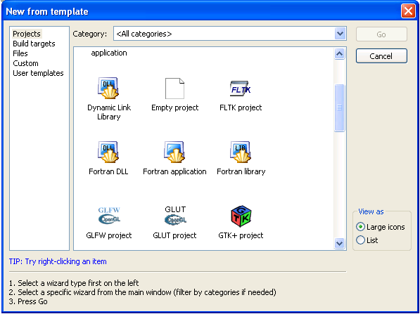
  1. Open code::blocks, and start a new project (File > New > Project) by selecting “Fortran application”newProject
  2. Provide a “Project title” and a location to store the files of the new project.setupProject1
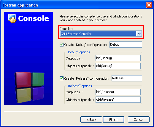
  3. Choose your compiler (GNU Fortran Compiler, make sure this is the one selected) and Finish.setupProject2
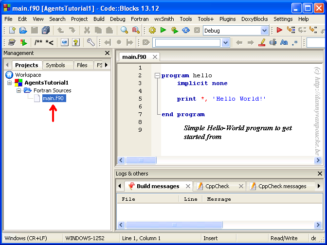
  4. Now Code::Blocks will present you a new project, with already one file present: main.f90 HelloWorld
  5. First we are going to rename this main file, e.g. to main.f95, to indicate that we will be  using Fortran 95 code in this file. By right-clicking on the file name (indicated with the red arrow) you see a list of possible op w this option while the file is open in the right-hand pane. Close the file there, and now you can rename main.f95.
  6. Although we will be following the OOP paradigm for the main internal workings of our program, a procedural setup will be used to set up the global lines of the program. I split the code in three levels: The top-level being the main program loop which is limited to the code below, the middle level which contains what you may normally consider the program layout (which you can easily merge with the top level) and the bottom level which contains the OO innards of our program. All subroutines/functions belonging to the middle level will be placed in one external module (Tutorial1) which is linked to the main program through the use-statement at line 2 and the single subroutine call (RunTutorial1).

[codesyntax lang=”fortran” lines=”normal” title=”Main-program” blockstate=”expanded”]

program AgentTutorials
    use Tutorial1;
    implicit none

    write(*,'(A)') "Welcome to the Agents OOP-Fortran Tutorial"
    call RunTutorial1()
    write(*,'(A)') "-- Goodbye"
end program AgentTutorials

[/codesyntax]

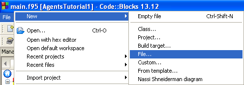
  1. Next step, we need a place for the RunTutorial1 subroutine, and all other subroutines/functions that will provide the global layout of our agents-program. Make a new file in Code::Blocks as followsNewFile
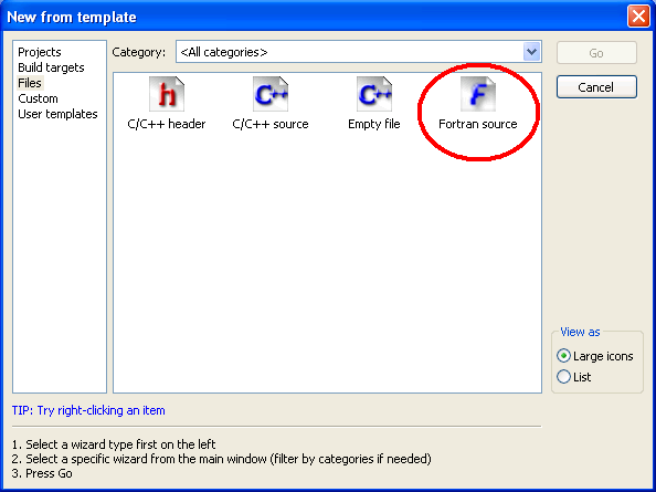
  2. and select a Fortran source file and finish by placing it in a directory of your choice and click OK.NewFile2
  3. In this empty file, a module is setup in the following fashion:

[codesyntax lang=”fortran” lines=”normal” strict=”yes” title=”Tutorial1.f95″ blockstate=”expanded”]

module Tutorial1
    implicit none
    private

    public :: RunTutorial1

 contains
    !+++++++++++++++++++++++++++++++++++++
    !>\brief Main program routine for the first agents tutorial
    !!
    !! This is the only function accessable outside this module.
    !<------------------------------------
    subroutine RunTutorial1()
        write(*,'(A)') "----Starting Turorial 1 subprogram.----"
        write(*,'(A)') "-------End Turorial 1 subprogram.------"
    end subroutine RunTutorial1

end module Tutorial1

[/codesyntax]

  1. implicit none : Makes sure that you have to define all variables.
  2. private : The private statement on line 3 makes sure that everything inside the module remains hidden for the outside world, unless you explicitly make it visible. In addition to data/information-hiding this also helps you keep your namespace in check.
  3. public :: Runtutorial1 : Only the function Runtutorial1 is available outside this module.(Because we want to use it in program  AgentTutorials.)
  4. contains : Below this  keyword all functions and subroutines of the module will be placed.
  5. “!” : The exclamation marks indicate a comment block. In this case it is formatted to be parsed by doxygen.
  6. subroutine XXX  / end subroutine XXX : The subroutine we will be implementing/using as the main loop of our agents program. Note that in recent incarnations of fortran the name of the subroutine/function/module/… is repeated at their end statement. For small functions this may look ridiculous, but for larger subroutines it improves readability.

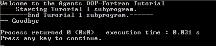
At this point or program doesn’t do that much, we have only set up the framework in which we will be working. Compiling and running the program (F9 or Build > Build and run) should show you:

AgentsRun1 In the next session of this tutorial we will use OO-Fortran 2003 to create the agent-class and create a first small simulation.


Permanent link to this article: https://dannyvanpoucke.be/oop-fortran-tut1-en/

Spring School Computational Tools: Day 5 – CP2K

Today was the fifth and last day of our spring school on computational tools for materials science. However, this was no reason to sit back and relax. After having been introduced into VASP (day-2) and ABINIT (day-3) for solids, and into Gaussian (day-4) for molecules, today’s code (CP2K) is one which allows you to study both when focusing on dynamics and solvation.

ensembles

If ensembles were coffee…

The introduction into the Swiss army knife called CP2K was provided by Dr. Andy Van Yperen-De Deyne. He explained to us the nature of the CP2K code (periodic, tools for solvated molecules, and focus on large/huge systems) and its limitations. In contrast to the codes of the previous days, CP2K uses a double basis set: plane waves where the properties are easiest and most accurate described with plane waves and gaussians where it is the case for gaussians. By means of some typical topics of calculations, Andy explained the basic setup of the input and output files, and warned for the explosive nature of too long time steps in molecular dynamics simulations. The possible ensembles for molecular dynamics (MD) were explained as different ways to store hot coffee. Following our daily routine, this session was followed by a hands-on session.

In the afternoon, the advanced session was presented by a triumvirate:  Thierry De Meyer, who discussed QM/MM simulations in detail, Dr. Andy Van Yperen-De Deyne, who discused vibrational finger printing and Lennart Joos, who, as the last presenter of the week, showed how different codes can be combined within a single project, each used where they are at the top of their strength, allowing him to unchain his zeolites.

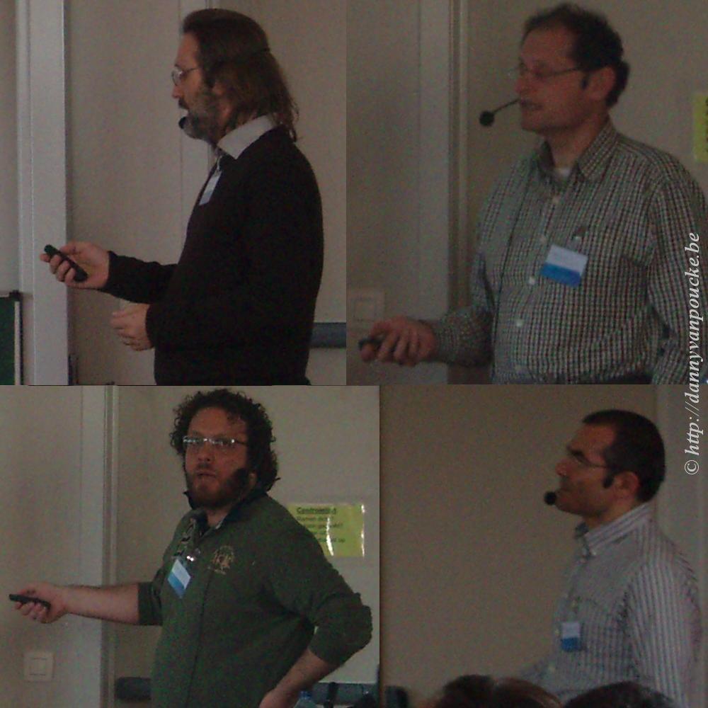
CP2K, all lecturers

CP2K, all lecturers: Andy Van Yperen-De Deyne (top left), Thierry De Meyer (top right), Lennart Joos (bottom left). All spring school participants hard at work during the hands-on session, even at this last day (bottom right).

The spring school ended with a final hands-on session on CP2K, where the CMM team was present for the last stretch, answering questions and giving final pointers on how to perform simulations, and discussing which code to be most appropriate for each project. At 17h, after my closing remarks, the curtain fell over this spring school on computational tools for materials science. It has been a busy week, and Kurt and I are grateful for the help we got from everyone involved in this spring school, both local and external guests. Tired but happy I look back…and also a little bit forward, hoping and already partially planning a next edition…maybe in two years we will return.

Guests from the VASP (Martijn Marsman, top left) and ABINIT group (Xavier Gonze, top right, Matteo Giantomassi, bottom left, Gian-Marco Rignanese, bottom right)

Our external lecturers from the VASP group (Martijn Marsman, top left) and the ABINIT group (Xavier Gonze, top right, Matteo Giantomassi, bottom left, Gian-Marco Rignanese, bottom right)

Permanent link to this article: https://dannyvanpoucke.be/ssct-day5-cp2k/

Spring School Computational Tools: Day 4 – Gaussian

After having focused on solids during the previous two days of our spring school, using either VASP (Tuesday) or ABINIT (Wednesday), today’s focus goes to molecules, and we turn our attention to the Gaussian code.

Dietmar Hertsen introduced us into the Gaussian code, and immediately showed us why this code was included in our spring school set: it is the most popular code (according to google). He also explained this code is so popular (among chemists) because it can do a lot of the chemistry chemists are interested in, and because of the simplicity of the input files for small molecules. After pointing out the empty lines quirks of Gaussian it was time to introduce some of the possible editors to use with Gaussian. The remainder of his lecture, Dietmar showed us how simple (typical) Gaussian calculations are run, pointing out interesting aspects of the workflow, and the fun of watching vibrations in molden. He ended his lecture giving us some tips and tricks for the investigation of transition states, and the study of chemical reactions, as a mental preparation for the first hands-on session which followed after the coffee-break.

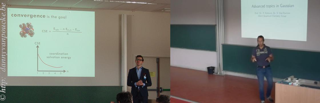
Lecturers for the Gaussian code.

Lecturers for the Gaussian code: Dietmar Hertsen (left) introducing the basics of the code, while Patrick Bultinck (right) discuses more advanced wave function techniques in more detail.

In the afternoon it was time to take out the big guns. Prof. Patrick Bultinck, of the Ghent Quantum Chemistry Group, was so kind to provide the advanced session. In this session, we were reminded, after two days of using the density as a central property, that wave functions are the only way to obtain perfect results. Unfortunately, practical limitations hamper the application to the systems of interest from a practical physical point of view. Patrick, being a quantum chemist to the bone, at several points stepped away from his slides and showed on the blackboard how several approximations to full configuration interaction (full-CI) can be obtained. He also made us aware of the caveats of such approaches; Such as size consistency and basis(-type) dependence for truncated CI, and noted that although CASSCF is a powerful method (albeit not for the fainthearted), it is somewhat a black art that should be used with caution. As such, CASSCF was not included in the advanced hands-on sessions guided by Dr. Sofie Van Damme (but who knows what may happen in a future edition of this spring school).

Permanent link to this article: https://dannyvanpoucke.be/ssct-day4-gaussian/

Spring School Computational Tools: Day 3 – Abinit

Today is the third day of our spring school. After the introduction to VASP yesterday, we now turn our attention to another quantum mechanical level solid state code: ABINIT. This is a Belgian ab initio code (mainly) developed at the Université Catholique de Louvain (UCL) in Wallonia.

Since no-one at CMM has practical experience with this code and several of us are interested to learn more about this code, we were very pleased that the group of Prof. Xavier Gonze was willing to support this day in its entirety. During the morning introductory session Prof. Xavier Gonze introduced us into the world of the ABINIT code, for which the initial ideas stem from 1997. Since then, the program has grown to about 800.000 lines of fortran code(!) and a team of 50 people worldwide currently contribute to its development. Also in recent years, a set of python scripts have been developed providing a more user friendly interface (abipy) toward the users of the code. The main goal of the development of this interface, is to shift interest back to the physics instead of trying to figure out which keywords do the trick. We also learned that the ABINIT code is strongly inspired by the ‘free software’ model, and as such Prof. Xavier Gonze prefers to refer to the copyright of ABINIT as copyleft. This open source mentality seems also to provide strength to the code; leading to its large number of developers/contributors; which in turn leads to the implementation of a wide variety of basis-sets, functionals and methodologies.

After the general introduction, Dr. Matteo Giantomassi introduced the abipy python package. This package was especially developed for automating post-processing of ABINIT results, and automatically generating input files. In short, to make interaction with ABINIT easier. Matteo, however, also warned that this approach which makes the use of ABINIT much more black box, might confuse beginners, since a lot of magic is going on under the hood of the abipy scripts. However, his presence, and that of the rest of the ABINIT delegation made sure confusion was kept to a minimum during the hands-on sessions, for which we are very grateful.

After the lunch break, Prof.  Gian-Marco Rignanese and Prof. Xavier Gonze held a duo seminar on more advanced topics covering Density Functional Perturbation Theory and based on this spectroscopy and phonon calculations beyond the frozen phonon approach. Of these last aspects I really am interested in seeing how they cope with my Metal Organic Frameworks

Permanent link to this article: https://dannyvanpoucke.be/ssct-day3-abinit/

Spring School Computational Tools: Day 2 – VASP

On this second day of our spring school, the first ab initio solid state code is introduced: VASP, the Vienna Ab initio Simulation Package.

Having worked with this code for almost a full decade, some consider me an expert, and as such I had the dubious task of providing first contact with this code to our participants. Since all basic aspects and methods had already been introduced on the first day, I mainly focused on presenting the required input files and parameters, and showing how these should be tweaked for some standard type solid state calculations. Following this one-hour introduction, in which I apparently had not yet scared our participants too much, all participants turned up for the first hands-on session, where they got to play with the VASP program.

In the afternoon, we were delighted to welcome our first invited speaker, straight from the VASP-headquarters: Dr. Martijn Marsman. He introduced us to advanced features of VASP going beyond standard DFT. He showed the power (and limitations) of hybrid-functionals and introduced the quasi-particle approach of GW. We even went beyond GW with the Bethe-Salpeter equations (which include electron-hole interactions). Unfortunately, these much more accurate approaches are also much more expensive than standard DFT, but there is work being done on the implementation of a cubic scaling RPA implementation, which will provide a major step forward in the field of solid state science. Following this session, a second hands-on session took place where exercises linked to these more advanced topic were provided and eagerly tried by many of the more advanced participants.

Permanent link to this article: https://dannyvanpoucke.be/ssct-day-2-vasp/

Spring School Computational Tools: Day 1

Today our one-week spring school on computational tools for materials science kicked off. During this week, Kurt Lejaeghere and I host this spring school, which we have been busily organizing the last few months, intended to introduce materials scientists into the use of four major ab-initio codes (VASP, ABINIT, Gaussian and CP2K). During this first day, all participants are immersed in the theoretical background of molecular modeling and solid state physics.

springschool

Prof. Karen Hemelsoet presented a general introduction into molecular modeling, showing us which computational techniques are useful to treat problems of varying scales, both in space and time. With the focus going to the modeling of molecules she told us everything there is to know about the potential energy surface, (PES)  how to investigate it using different computational methods. She discussed the differences between localized (i.e. gaussian) and plane wave basis sets and taught us how to accurately sample the PES using both molecular dynamics and normal mode analysis. As a final topic she introduced us to the world of computational spectroscopy, showing how infrared spectra can be simulated, and the limitations of this type of simulations.

With the, somewhat mysterious, presentations of Prof. Stefaan Cottenier we moved from the  realm of molecules to that of solids. In his first session, he introduced density functional theory, a method ideally suited to treat extended systems at the quantum mechanical level. And showed that as much information is present in the electron density of a system as is in its wave function. In his second session, we fully plunged in the world of solids, and we were guided, step by step, towards a full understanding of the technical details generally found in the methods section of (ab-initio) computational materials science work. Throughout this session, NaCl was used as an ever present example, and we learned that our simple high-school picture of bonding in kitchen salt is a lie-to-children. In reality, Cl doesn’t gain an extra electron by stealing it away from Na, instead it is rather the Na 3s electron which is living to far away from the Na nucleus it belongs to.

Permanent link to this article: https://dannyvanpoucke.be/ssct-day1/

De-activating an active atom.

It could be that I’ve perhaps found out a little bit about the structure
of atoms. You must not tell anyone anything about it. . .
–Niels Bohr (1885 – 1965),
in a letter to his brother (1912)

Getting the news that a paper got accepted for publication is exciting news, but it can also be a little bit sad since it indicates the end of a project. Little over a month ago we got this great news regarding our paper for the journal of chemical information and modeling. It was the culmination of a side project Goedele Roos and I had been working on, in an on-and-off fashion, over the last two years.

When we started the project each of us had his/her own goal in mind. In my case, it was my interest in showing that my Hirshfeld-I code could handle systems which are huge from the quantum mechanical calculation point of view. Goedele, on the other hand, was interested to see how good Hirshfeld-I charges behaved with increasing size of a molecular fraction. This is of interest for multiscale modeling approaches, for which Martin Karplus, Michael Levitt, and Arieh Warshel got the Nobel prize in chemistry in 2013. In such an approach, a large system, for example a solvated biomolecule containing tens of thousands of atoms, is split into several regions. The smallest central region, containing the part of the molecule one is interested in is studied quantum mechanically, and generally contains a few dozen up to a few hundred atoms. The second shell is much larger, and is described by force-field approaches (i.e. Newtonian mechanics) and can contain ten of thousands of atoms. Even further  from the quantum mechanically treated core a third region is described by continuum models.

What about the behavior of the charges? In a quantum mechanical approach, even though we still speak of electrons as-if referring to classical objects, we cannot point to a specific point in space to indicate: “There it is”. We only have a probability distribution in space indicating where the electron may be. As such, it also becomes hard to pinpoint an atom, and in an absolute sense measure/calculate it’s charge. However, because such concepts are so much more intuitive, many chemists and physicists have developed methods, with varying success, to split the electron probability distribution into atoms again. When applying such a scheme on the probability distributions of fractions of a large biomolecule, we would like the atoms at the center not to change to much when the fraction is made larger (i.e. contain more atoms). This would indicate that from some point onward you have included all atoms that interact with the central atoms. I think, you can already see the parallel with the multiscale modeling approach mentioned above; where that point would indicate the boundary between the quantum mechanical and the Newtonian shell.
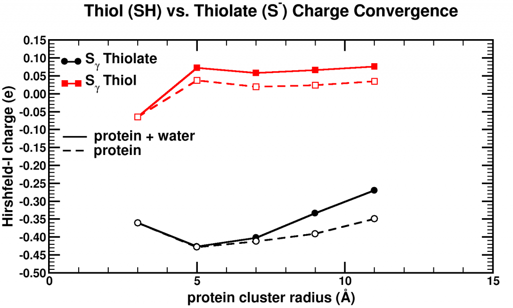
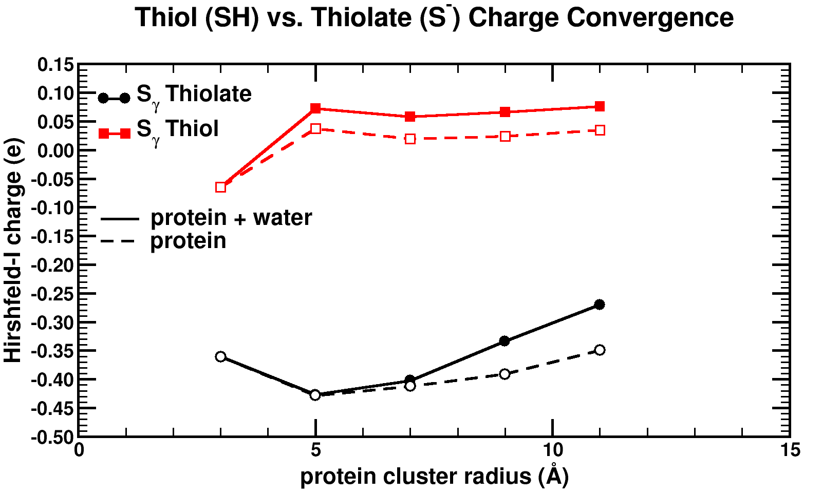
Convergence of Hirshfeld-i charges for clusters of varying size of a biomolecule.

Convergence of Hirshfeld-I charges for clusters of varying size of a biomolecule. The black curves show the charge convergence of an active S atom, while the red curves indicate a deactivated S atom.

Although, we expected to merely be studying this convergence behavior, for the particular partitioning scheme I had implemented, we dug up an unexpected treasure. Of the set of central atoms we were interested all except one showed the nice (and boring) convergence behavior. The exception (a sulfur atom) showed a clear lack of convergence, it didn’t even show any intend toward convergence behavior even for our system containing almost 1000 atoms. However, unlike the other atoms we were checking, this S atom had a special role in the biomolecule: it was an active site, i.e. the atom where chemical reactions of the biomolecule with whatever else of molecule/atom are expected to occur.

Because this S atom had a formal charge of -1, we bound a H atom to it, and investigated this set of new fractions. In this case, the S atom, with the H atom bound to it, was no longer an active site. Lo and behold, the S atom shows perfect convergence like all other atoms of the central cluster. This shows us that an active site is more than an atom sitting at the right place at the right time. It is an atom which is reaching out to the world, interacting with other atoms over a very long range, drawing them in (>10 ångström=1 nm is very far on the atomic scale, imagine it like being able to touch someone who is standing >20 m away from you). Unfortunately, this is rather bad news for multiscale modeling, since this means that if you want to describe such an active site accurately you will need an extremely large central quantum mechanical region. When the active site is deactivated, on the other hand, a radius of ~0.5 nm around the deactivated site is already sufficient.

Similar  to Bohr, I have the feeling that “It could be that I’ve perhaps found out a little bit about the structure
of atoms.”, and it makes me happy.

Permanent link to this article: https://dannyvanpoucke.be/de-activating-an-active-atom/

Start to Fortran

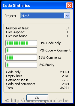
Code-statistics for the hive3 code (feb.2015)

Code-statistics for the hive3 code (feb.2015)

If you are used to programming in C/C++, Java or Pascal, you probably do this using an Integrated Development Environment (IDE’s) such as Dev-Cpp/Pascal, Netbeans, Eclipse, … There are dozens of free IDE’s for each of these languages. When starting to use fortran, you are in for a bit of a surprise. There are some commercial IDE’s that can handle fortran (MS Visual Studio, or the Lahey IDE). Free fortran IDEs are rather scarce and quite often are the result of the extension of a C++ focused IDE. This, however, does not make them less useful. Code::Blocks is such an IDE. It supports several programming and scripting languages including C and fortran, making it also suited for mixed languages development. In addition, this IDE has been developed for Windows, Linux and Mac Os X, making it highly portable. Furthermore, installing this IDE combined with for example the gcc compiler can be done quickly and without much hassle, as is explained in this excellent tutorial. In 5 steps everything is installed and you are up and running:

  1. Get a gfortran compiler at https://gcc.gnu.org/wiki/GFortran

    Go for binaries and get the installer if you are using Windows. This will provide you with the latest build. Be careful if you are doing this while upgrading from gfortran 4.8 to 4.9 or 4.10. The latter two are known to have a recently fixed compiler-bug related to the automatic finalization of objects. A solution to this problem is given in this post.

    UPDATE 03/02/2017: As the gcc page has changed significantly since this post was written, I suggest to follow the procedure described here for the installation of a 64bit version of the compiler.

  2. Get the Code::Blocks IDE at http://www.codeblocks.org/ or http://cbfortran.sourceforge.net/ (preferred)

    Since version 13.12 the Fortranproject plugin is included in the Code::Blocks installation.

  3. Setup gfortran

    Run the installer obtained at step 1…i.e. keep clicking OK until all is finished.

  4. Setup Code::Blocks for fortran
    1. Run the installer or Unzip the zip-file obtained in step 2.
    2. Run Code::Blocks and set your freshly installed GNU fortran compiler as default.
    3. Associate file types with Code::Blocks. If you are not using other IDE’s this may be an interesting idea
    4. Go to settings, select “Compiler and Debugger”, click on “Toolchain executables” and set the correct paths.
    5. Code::blocks has been configured.
  5. Your first new fortran program
    1. Go to “File” → “New” → “Project”.
    2. Select “Fortran Application”.
    3. Follow the Wizard: provide a project folder and title.
    4. Make sure the compiler is set to “GNU Fortran Compiler”, and click Finish.
    5. A new project is now being created, containing a main file named “main.f90”
    6. Click “Build”, to build this program, and then “Run”.
    7. Congratulations your first Fortran program is a fact.


Of course any real project will contain many files, and when you start to create fortran 2003/2008 code you will want to use “.f2003” or “.f03” instead of “.f90” . The Code::Blocks IDE is well suited for the former tasks, and we will return to these later. Playing with this IDE is the only way to learn about all its options. Two really nice plugins are “Format Fortran Indent” and “Code statistics”. The first one can be used to auto-indent your Fortran code, making it easier to find those nasty missing “end” statements. The code statistics tool runs through your entire project and tells you how many lines of code you have, and how many lines contain comments.

Permanent link to this article: https://dannyvanpoucke.be/start-to-fortran-en/