Fine-tuning the theoretically predicted structure of MIL-47(V) with the aid of powder X-ray diffraction

Authors: Thomas Bogaerts, Louis Vanduyfhuys, Danny E. P. Vanpoucke, Jelle Wieme,
Michel Waroquier, Pascal van der Voort and Veronique van Speybroeck
Journal: Cryst. Eng. Comm. 17(45), 8612-8622 (2015)
doi: 10.1039/c5ce01388g
IF(2015): 3.849
export: bibtex
pdf: <Cryst.Eng.Comm.> 
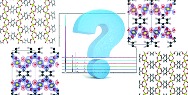
Graphical Abstract: Which model represents the experimental XRD-spectra best? Ferromagnetic or anti-ferromagnetic chains? With of without offset?
Graphical Abstract: Which model represents the experimental XRD-spectra best? Ferromagnetic or anti-ferromagnetic chains? With of without offset?

Abstract

The structural characterization of complex crystalline materials such as metal organic frameworks can prove a very difficult challenge both for experimentalists as for theoreticians. From theory, the flat potential energy surface of these highly flexible structures often leads to different geometries that are energetically very close to each other. In this work a distinction between various computationally determined structures is made by comparing experimental and theoretically derived X-ray diffractograms which are produced from the materials geometry. The presented approach allows to choose the most appropriate geometry of a MIL-47(V) MOF and even distinguish between different electronic configurations that induce small structural changes. Moreover the techniques presented here are used to verify the applicability of a newly developed force field for this material. The discussed methodology is of significant importance for modelling studies where accurate geometries are crucial, such as mechanical properties and adsorption of guest molecules.

Permanent link to this article: https://dannyvanpoucke.be/paper2015_xrd_crystendcomm-en/

IAP-meeting 2015: poster

Falling ill is always a bummer. It’s even more annoying when you just finished preparing a poster for a conference you intended to attend (in the current case this is the annual IAP meeting). Per doctor’s orders I am not allowed to be patient zero at the above conference, so my poster will end up alone at the site (luckily my nice colleagues will take it along and put it up). Because misery loves company (or it’s just a personal skill to pick the wrong moment) I had also decided to make this poster a bit more interactive through a spartan setup: As little text as possible, only a trail of images through  which I would tell the story of the research…As you can see I was asking for trouble.

Not being able to be there physically, and knowing that most people nowadays own a smart-phone, I came up with the following solution: One of my colleagues will also put up a QR-code, sending the interested reader to this blog-post, where he/she will be able to read the story of the poster. (Questions can be put in the comments, and the full size version of the poster can be reached by clicking on the picture below.)

Abstract

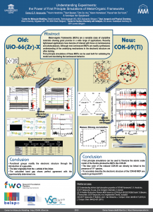
Poster created for the 2015 IAP meeting on september 11<SUP>th</SUP>, 2015 in Hasselt, Belgium.

Poster created for the 2015 IAP meeting on September 11th, 2015 in Hasselt, Belgium.

Metal-Organic Frameworks (MOFs) are a versatile class of crystalline materials showing great promise in a wide range of applications. Recently, light-based applications, with a focus on luminescence and photo-catalysis, have become of interest. Although new luminescent MOFs are readily synthesized, a fundamental understanding of the underlying mechanisms in the electronic structure is often lacking.

First principles, or ab initio simulations of these MOFs can be used both for validating the experimentally proposed atomistic model of the MOF and for elucidating its luminescent behavior. On this poster, two different MOF-topologies are investigated. In the first case, we consider the well-known UiO-66(Zr) MOF. For this MOF, it is known that functionalization of the linkers modifies its luminescent behavior. As our second case, we consider the very recently created/synthesized COK-69(Ti) MOF. This new MOF is both flexible and luminescent, making it of interest for various applications.

The Old: UiO-66(Zr)-X

Atomic Structure

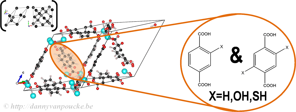
In our work on the UiO-66, we made use of the primitive unit cell, which contains only a single node and six linker molecules. This cell still contains about 120 atoms (in contrast to about 480 atoms for the conventional cubic cell) making it a rather large system from the point of view of ab initio calculations. The relation between this primitive unit cell and the conventional cubic cell is indicated by comparison to the diamond primitive and cubic cell (top left corner).

The functionalized versions of this MOF were created by manually replacing some of the H atoms of the BDC-linker (benzene-1,4-dicarboxylic acid) by the functional group of interest (OH or SH) and then optimizing the entire structure.

Ball-and-stick model of a primitive unit cell of UiO-66.

Ball-and-stick model of a primitive unit cell of UiO-66(Zr). Linker functionalization is indicated on the right. Primitive and conventional unit cells for diamond are given as reference.

Electronic Structure

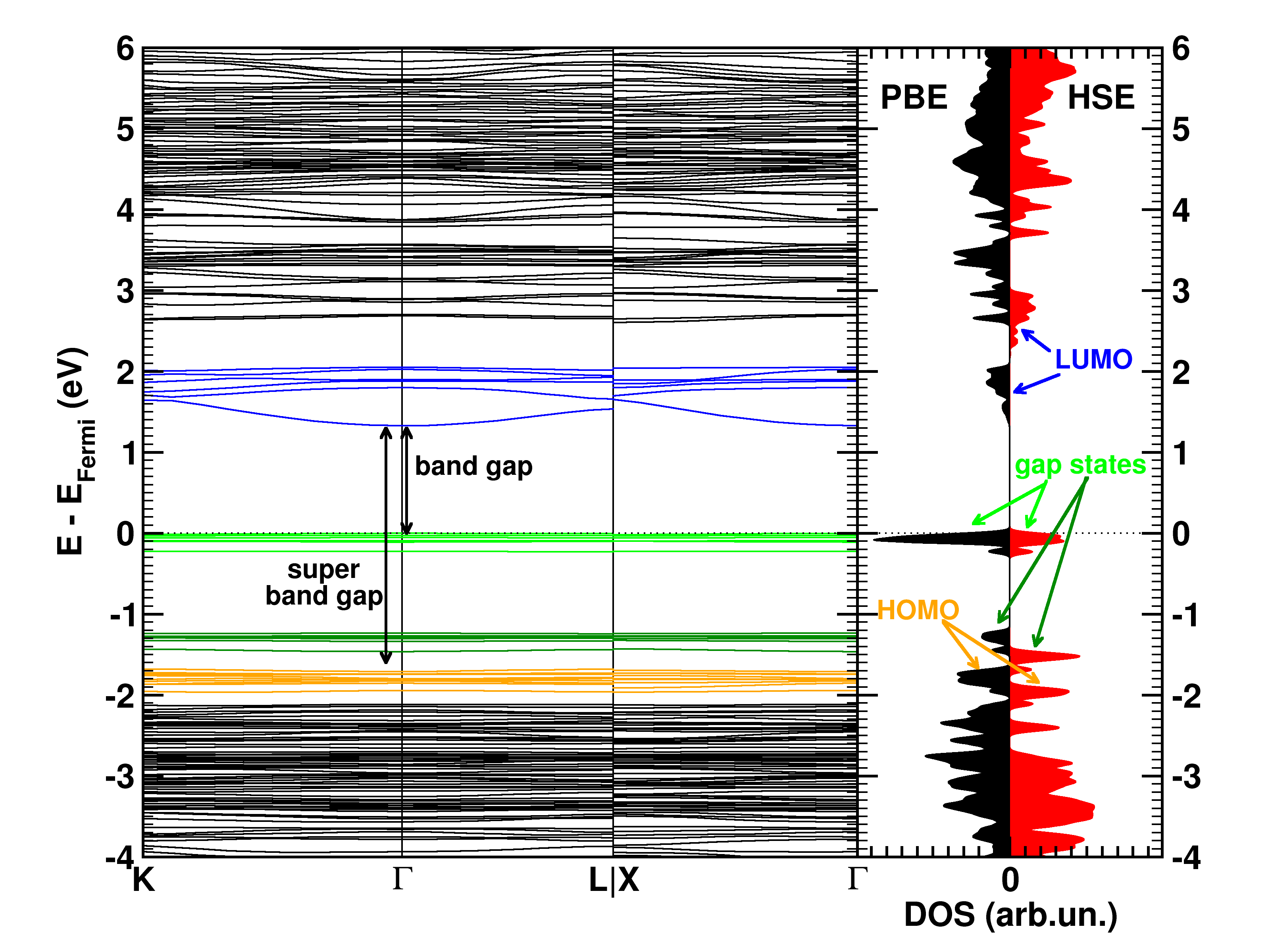
Electronic band structure and DOS of UiO-66(Zr)-2,5SH

The calculated electronic band structure (left) and density of states (right) of the double SH-functionalized UiO-66(Zr). The conduction band is colored in blue, while the gap states related to the functional groups are colored green. The “old” valence band is colored yellow. This picture is a modified version of the published one.(Ref 1)

Starting from the optimized geometrical structures, the electronic structure is investigated. Taking three high-symmetry lines of the first Brillouin zone, the band structure was generated for all the functionalized MOFs.

The first aspect that drew my attention was the fact that the bottom conduction bands (indicated in blue) remained unchanged while part of the top of the valence band (indicated in green) splits off and moved upward into the band gap. At this point, nomenclature also becomes a bit of a problem. In a doped semi-conductor, the green bands would be called gap states, which would mean that the band gap of the host-material remains unchanged (which is actually also the case here, the distance between the yellow valence band and the blue conduction band is exactly the same for all functionalized UiO-66(Zr) systems we investigated). However, unlike those semiconductors, these gap states are entirely filled, and contain a significant electron occupation (in doped semi-conductors, these states often appear due to ppm doping). Because of this, they take the role of the valence band leading to a measured band gap equal to the distance between the top green bands and the conduction band (blue). So we end up with two band gaps. To have a clear link with experiments on MOFs, we will call the latter the band gap, while we will call the distance between the yellow and blue bands the “super band gap” (super, to indicate that we go beyond the size of the band gap, but it can still be considered a band gap. If that were not the case, we should call it the “supra band gap”).

The discussion of the super band gap can be rather short: it remains unchanged from the value of the unfunctionalized UiO-66(Zr): roughly 4 eV. In contrast, the band gap depends on both the functional group, and the number of functional groups present on each linker. In case of the double SH-functionalized linkers, each functional group leads to a gap state that is being split of from the valence band (cf. two green bands in the right picture).

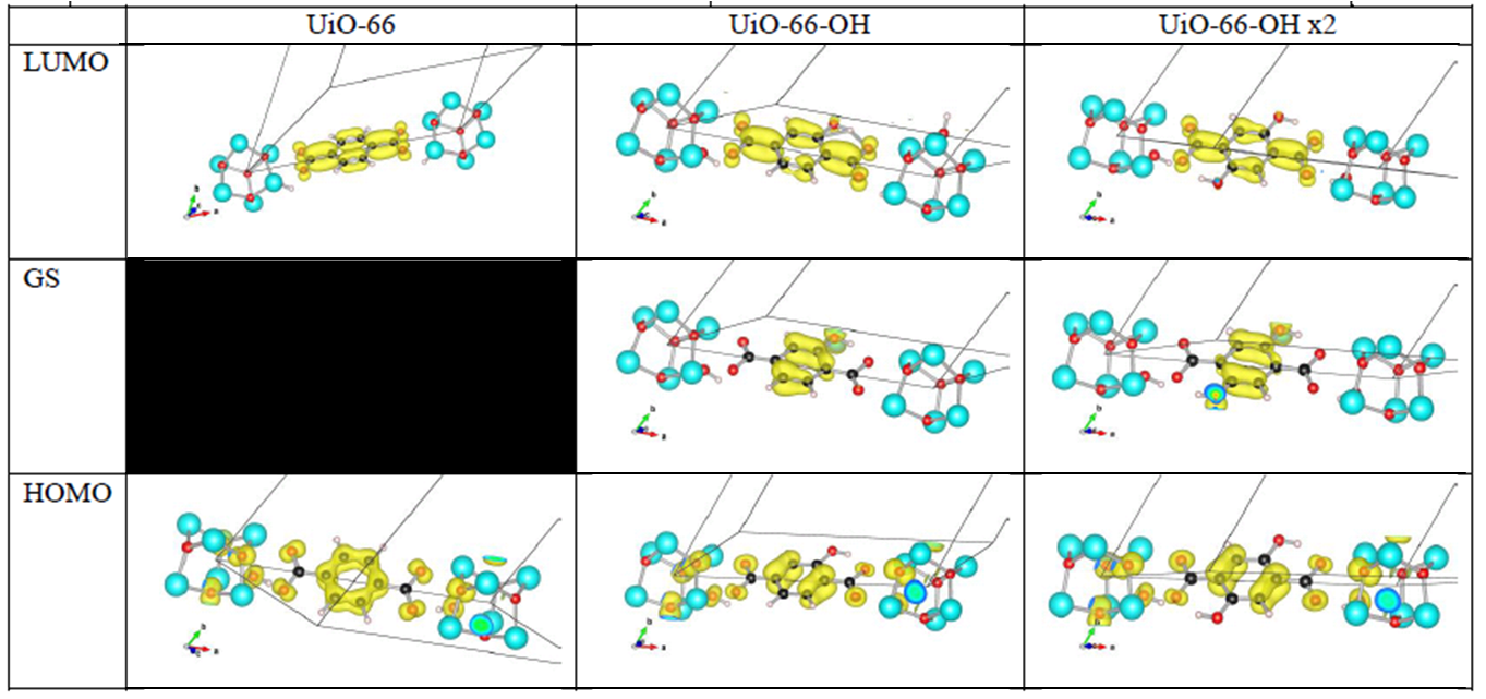
Orbital character of valence and conduction band.

Orbital character of gap states, and valence and conduction bands for OH functionalized linkers in UiO-66(Zr).

Analysis of the orbital character shows that the splitting of the valence band can be taken quite literal. Where the valence band (or HOMO if you use molecular terminology) of the unfunctionalized UiO-66(Zr) mainly consists of the π-orbital of the BDC linker, this orbital is split upon functionalization. The conduction band orbital (or LUMO) on the other hand is barely modified.

Because LDA and GGA functionals are well-known to underestimate the experimental band gaps (even though the band structure is qualitatively well represented), we have also used a hybrid functional (HSE06, which was developed for solids) to calculate the band gap, and as expected, we find that the qualitative picture of the electron density of states (DOS) is retained, and the resulting calculated band gap is in perfect agreement with the experimentally measured values (experiments performed by Kevin Hendrickx of the Centre for Ordered Materials, Organometallics and Catalysis at Ghent University).

In conclusion, our ab initio calculations have shown us that functionalization of the linkers leads to a splitting of the valence band and the creation of a gap state, and that the band gap can be predicted with great accuracy for these materials.

The New: COK-69(Ti)

Atomic Structure

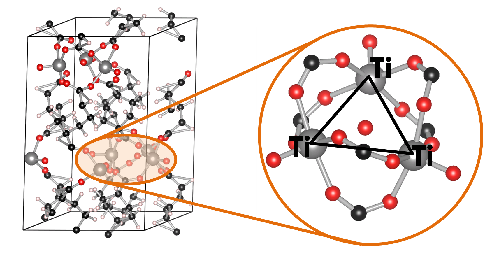
Ball-and-stick model of the COK-69(Ti) MOF.

Ball-and-stick model of the COK-69(Ti) MOF. A single triangular Ti cluster is shown in more detail.

The COK-69(Ti) MOF is a newly developed MOF by the Center for Surface Chemistry and Catalysis of the university of Leuven. It is one of the few Ti containing MOFs that have already been synthesized. Because of this, the initial model provided was not sufficiently accurate to perform good electronic structure calculations. The weak point of the model was the uncertainty of the actual structure of the triangular Ti-O clusters. The original model (figure a) was not charge balanced. As a result, the electronic structure of this model showed it to be a metal (or a very narrow band gap semiconductor), in clear disagreement with experiment. Charge balance could be obtained in several ways: removal of O atoms, formation of H2O bound to the cluster (e.g. figure c) or the formation of OH groups (e.g. figure b). By investigating different models, we found that the removal of O atoms is highly unfavorable, while the formation of OH groups and a bound H2O molecule are comparable in stability. As a result of the latter observation, it is not unreasonable to assume that under experimental conditions the bound H2O molecule dissociates and lead to the formation of two OH groups, and that this process is also reversed, leading to a constant moving back and forth between the two models.

Models for Ti clusters in the COK-69(Ti) MOF.

Schematic representation of possible triangular Ti clusters for the CO-69(Ti) MOF.

Electronic Structure

Also, the calculated electronic structure for both models is reasonably comparable: similar sized band gaps, and the same character for the valence (mainly O states) and the conduction (mainly Ti states) bands. Making it hard to give preference to one model over the other as being the actual ground state structure of this MOF, without further study.

Irradiated COK-69

More interestingly, we found the cluster with three OH groups (cf. figure d) to be most stable. In such a model, two of the Ti atoms should have an oxidation number of 4, while one has an oxidation number of 3. Looking into the electronic structure of this specific model of the COK-69 shows some amazing features. Firstly, the band gap is much reduced to about the size associated with a semiconductor, and secondly, the states of the Ti3+ atom show a valence to conduction transition of 3.2 eV, which roughly coincides with the blue color obtained for the irradiated COK-69 MOF.

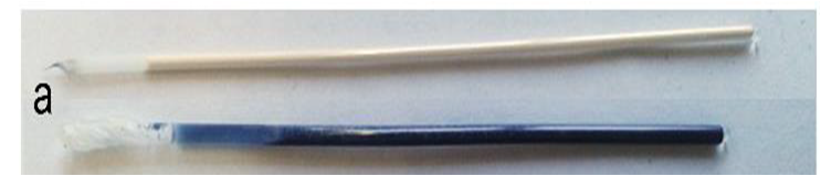
Samples of the COK-69(Ti) MOF.

Two samples of the COK-69(Ti) MOF. The normal COK-69 at the top, and the irradiated COK-69 MOF at the bottom. Figure taken from Ref 2.

Ti3+ centers are known to provide a blue color in other materials, and it is now also shown to be the case for this MOF. In addition, experiments on the irradiated COK-69 MOF also showed that no more than 1/3 of the Ti atoms could be Ti3+, which is also the maximum indicated by our model (one Ti per Ti-cluster).

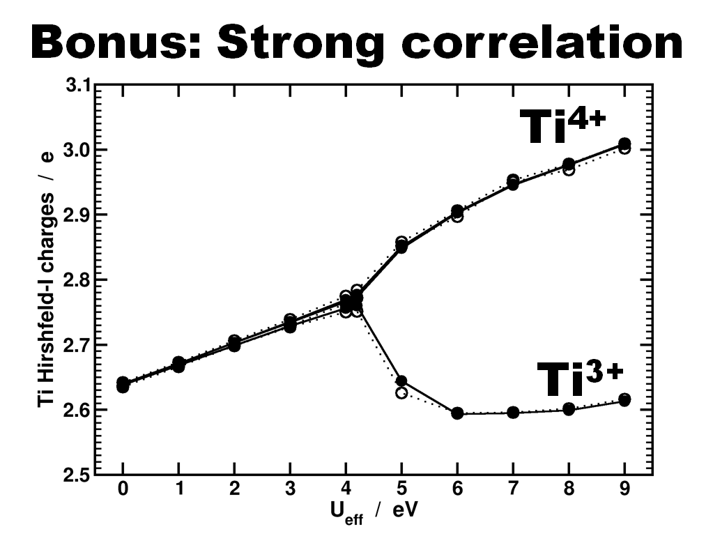
Another interesting bonus provided by this last model is from the theoretical perspective. Due to the symmetry of the cluster and the strong correlation of the Ti-d states, standard DFT is not able to differentiate between the Ti4+ and Ti3+ atoms. As such, the atomic charge is the same for all. By adding an additional Hubbard U potential on the Ti-d states (the so-called DFT+U approach) it is possible to differentiate between the different Ti oxidation states, as is shown by the nice bifurcation diagram.

Differentiation of Ti species.

Differentiation of Ti species as function of the U value used in a DFT+U approach. Atomic charges are calculated using the Hirshfeld-I partitioning scheme[3]. Figure taken from Ref 2.

In conclusion, our ab initio calculations allowed us to build a more accurate model of the COK-69 MOF and provide a model for the irradiated COK-69 MOF. In case of the latter, the calculated electronic structure can be used to elucidate the blue color of the irradiated COK-69.

References

[1] “Understanding intrinsic light absorption properties of UiO-66 frameworks”, K. Hendrickx, D.E.P. Vanpoucke, K. Leus, et al.  Inorganic Chemistry (in revision)

[2] “A Flexible Photoactive Titanium MOF based on a [TiIV3(µ3-O)O2(COO)6]-Cluster”, B. Beuken, F. Vermoortele, D.E.P. Vanpoucke, et al. Angewandte Chemie (accepted)

[3] D.E.P. Vanpoucke, P. Bultinck, and I. Van Driessche, J. Comput. Chem. 34 405-417 (2013) & J. Comput. Chem. 34 422-427 (2013)

Permanent link to this article: https://dannyvanpoucke.be/iap-meeting-poster-2015-en/

Fortran dll’s and libraries: a Progress bar

In the previous fortran tutorials, we learned the initial aspects of object oriented programming (OOP) in fortran 2003. And even though our agent-based opinion-dynamics-code is rather simple, it can quickly take several minutes for a single run of the program to finish. Two tools which quickly become of interest for codes that need more than a few minutes to run are: (1) a progress bar, to track the advance of the “slow” part of the code and prevent you from killing the program 5 seconds before it is to finish, and (2) a timer, allowing you to calculate the time needed to complete certain sections of code, and possibly make predictions of the expected total time of execution.

In this tutorial, we will focus on the progress bar. Since our (hypothetical) code is intended to run on High-Performance Computing (HPC) systems and is written in the fortran language, there generally is no (or no easy) access to GUI’s. So we need our progress bar class to run in a command line user interface. Furthermore, because it is such a widely useful tool we want to build it into a (shared) library (or dll in windows).progress_1pct

The progress bar class

What do we want out of our progress bar? It needs to be easy to use, flexible and smart enough to work nicely even for a lazy user. The output it should provide is formatted as follows: <string> <% progress> <text progress bar>, where the string is a custom character string provided by the user, while ‘%progress’ and ‘text progress bar’ both show the progress. The first shows the progress as an updating number (fine grained), while the second shows it visually as a growing bar (coarse grained).

[codesyntax lang=”fortran” lines=”normal” title=”TProgressBar Class” bookmarkname=”PBarClass” blockstate=”expanded” doclinks=”0″]

type, public :: TProgressBar
        private
        logical :: init
        logical :: running
        logical :: done
        character(len=255) :: message
        character(len=30) :: progressString
        character(len=20) :: bar
        real :: progress
    contains
        private
        procedure,pass(this),public :: initialize
        procedure,pass(this),public :: reset
        procedure,pass(this),public :: run
        procedure,pass(this),private:: printbar
        procedure,pass(this),private:: updateBar
    end type TProgressBar

[/codesyntax]

All properties of the class are private (data hiding), and only 3 procedures are available to the user: initialize, run and reset. The procedures, printbar and updatebar are private, because we intend the class to be smart enough to decide if a new print and/or update is required. The reset procedure is intended to reset all properties of the class. Although one might consider to make this procedure private as well, it may be useful to allow the user to reset a progress bar in mid progress.(The same goes for the initialize procedure.)

[codesyntax lang=”fortran” lines=”normal” title=”Run procedure of the TProgressBar class” blockstate=”expanded” bookmarkname=”RunProcedure” ]

subroutine run(this,pct,Ix,msg)
        class(TProgressBar) :: this
        real::pct
        integer, intent(in), optional :: Ix
        character(len=*),intent(in),optional :: msg

        if (.not. this%init) call this%initialize(msg)
        if (.not. this%done) then
            this%running=.true.
            this%progress=pct
            call this%updateBar(Ix)
            call this%printbar()
            if (abs(pct-100.0)<1.0E-6) then
                this%done=.true.
                write(*,'(A6)') "] done"
            end if
        end if

    end subroutine run

[/codesyntax]

In practice, the run procedure is the heart of the class, and the only procedure needed in most applications. It takes 3 parameters: The progress (pct), the number of digits to print of pct (Ix),and the <string> message (msg). The later two parameters are even optional, since msg may already have been provided if the initialize procedure was called by the user. If the class was not yet initialized it will be done at the start of the procedure. And while the progress bar has not yet reached 100% (within 1 millionth of a %) updates and prints of the bar are performed. Using a set of Boolean properties (init, running, done), the class keeps track of its status. The update and print procedures just do this: update the progress bar data and print the progress bar. To print the progress bar time and time again on the same line, we need to make use of the carriage return character (character 13 of the ASCII table):

write(*,trim(fm), advance='NO') achar(13), trim(this%message),trim(adjustl(this%progressString)),'%','[',trim(adjustl(this%bar))

The advance=’NO‘ option prevents the write statement to move to the next line. This can sometimes have the unwanted side-effect that the write statement above does not appear on the screen. To force this, we can use the fortran 2003 statement flush(OUTPUT_UNIT), where “OUTPUT_UNIT” is a constant defined in the intrinsic fortran 2003 module iso_fortran_env. For older versions of fortran, several compilers provided a (non standard) flush subroutine that could be called to perform the same action. As such, we now have our class ready to be used. The only thing left to do is to turn it into a dll or shared library.progress_25pct

How to create a library and use it

There are two types of libraries: static and dynamic.

Static libraries are used to provide access to functions/subroutines at compile time to the library user. These functions/subroutines are then included in the executable that is being build. In linux environments these will have the extension “.a”, with the .a referring to archive. In a windows environment the extension is “.lib”, for library.

Dynamic libraries are used to provide access to functions/subroutines at run time. In contrast to static libraries, the functions are not included in the executable, making it smaller in size. In linux environments these will have the extension “.so”, with the .so referring to shared object. In a windows environment the extension is “.dll”, for dynamically linked library.

In contrast to C/C++, there is relatively little information to be found on the implementation and use of libraries in fortran. This may be the reason why many available fortran-“libraries” are not really libraries, in the sense meant here. Instead they are just one or more files of fortran code shared by their author(s), and there is nothing wrong with that. These files can then be compiled and used as any other module file.

So how do we create a library from our Progressbar class? Standard examples start from a set of procedures one wants to put in a library. These procedures are put into a .f or .f90 file. Although they are not put into a module (probably due to the idea of having compatibility with fortran 77) which is required for our class, this is not really an issue. The same goes for the .f03 or .f2003 extension for our file containing a fortran 2003 class. To have access to our class and its procedures in our test program, we just need to add the use progressbarsmodule clause. This is because our procedures and class are incorporated in a module (in contrast to the standard examples). Some of the examples I found online also include compiler dependent pragmas to export and import procedures from a dll. Since I am using gfortran+CB for development, and ifort for creating production code, I prefer to avoid such approaches since it hampers workflow and introduces another possible source of bugs.

The compiler setups I present below should not be considered perfect, exhaustive or fool-proof, they are just the ones that work fine for me. I am, however, always very interested in hearing other approaches and fixes in the comments.progress_52pct

Windows

The windows approach is very easy. We let Code::Blocks do all the hard work.

shared library: PBar.dll

Creating the dll : Start a new project, and select the option “Fortran DLL“. Follow the instructions, which are similar to the setup of a standard fortran executable. Modify/replace/add the fortran source you wish to include into your library and build your code (you can not run it since it is a library).

Creating a user program : The program in which you will be using the dll is setup in the usual way. And to get the compilation running smoothly the following steps are required:

  • Add the use myspecificdllmodule clause where needed, with myspecificdllmodule the name of the module included in the dll you wish to use at that specific point.
  • If there are modules included in the dll, the *.mod files need to be present for the compiler to access upon compilation of the user program. (Which results in a limitation with regard to distribution of the dll.)
  • Add the library to the linker settings of the program (project>build options>linker settings), and then add the .dll file.
  • Upon running the program you only need the program executable and the dll.

static library

The entire setup is the same as for the shared library. This time, however, choose the “Fortran Library” option instead of Fortran dll. As the static library is included in the executable, there is no need to ship it with the executable, as is the case for the dll.

Unix

For the unix approach we will be working on the command line, using the intel compiler, since this compiler is often installed at HPC infrastructures.

static library: PBar.a

After having created the appropriate fortran files you wish to include in your library (in our example this is always a single file: PBar.f03, but for multiple files you just need to replace PBar.f03 with the list of files of interest.)

  1. Create the object files:
    ifort -fpic -c -free -Tf Pbar.f03

    Where -fpic tells the compiler to generate position independent code, typical for use in a shared object/library, while -c tells the compiler to create an object file. The -free and -Tf compiler options are there to convince the compiler that the f03 file is actual fortran code to compile and that it is free format.

  2. Use the GNU ar tool to combine the object files into a library:
    ar rc PBarlib.a PBar.o
  3. Compile the program with the library
    ifort TestProgram.f90 PBarlib.a -o TestProgram.exe

    Note that also here the .mod file of our Progressbarsmodule needs to be present for the compilation to be successful.

shared library: PBar.so

For the shared library the approach does not differ that much.

  1. Create the object files:
    ifort -fpic -c -free -Tf Pbar.f03

    In this case the fpic option is not optional in contrast to the static library above. The other options are the same as above.

  2. Compile the object files into a shared library:
    ifort -shared PBar.o -o libPBar.so

    The compiler option -shared creates a shared library, while the -o option allows us to set the name of the library.

  3. Compile the program with the library
    ifort TestProgram.f90 libPBar.so -o TestProgram.exe

    Note that also here the .mod file of our Progressbarsmodule needs to be present for the compilation to be successful. To run the program you also need to add the location of the library file libPBar.so to the environment variable LD_LIBRARY_PATH

One small pickle

HPC systems may perform extensive buffering of data before output, to increase the efficiency of the machine (disk-writes are the slowest memory access option)…and as a result this can sometimes overrule our flush command. The progressbar in turn will not show much progress until it is actually finished, at which point the entire bar will be shown at once. There are options to force the infrastructure not to use this buffering (and the system administrators in general will not appreciate this), for example by setting the compiler flag -assume nobuffered_stdout. So the best solution for HPC applications will be the construction of a slightly modified progress bar, where the carriage return is not used.

progress_100pct


Special thanks also to the people of stack-exchange for clarifying some of the issues with the modules.

Source files for the class and test-program can be downloaded here.


Permanent link to this article: https://dannyvanpoucke.be/fortran-dlls-en/

Stargazing at the ISS

What happens if two physicists take a holiday? They end up stargazing and hunting for the International Space Station (ISS). During the last week and a half we tried to capture the ISS flybys on camera nearly every night (with varying success). Each night we learned new things:

ISS and starscape

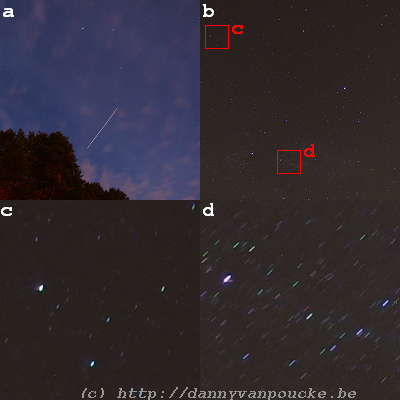
(a) Flyby of the ISS on August 4, 22h38 with a 20 second exposure, and ISO speed of 160. (b) Midnight starscape on august 5th (awaiting the ISS flyby) with a 60 second exposure at ISO-160. (c) and (d) zoomed in sections of (b) showing the color of the stars and arcs due to the earth rotation. (c) shows the a section of sky quite close to the north(small arcs). The arcs shown in (d) are about 15 arc-minute in size. (pictures by Sylvia Wenmackers)

  • Prolonged exposure photography makes night-sky pictures very interesting:
    • The overall sky quickly becomes overexposed (the least bit of final sunlight even after sunset, and the sky turn bright like it is midday, cf. picture (a))
    • Stars truly have colors you can see.(I’m a city boy, and even though as a physicist I am well aware of this it didn’t really fully register before I saw our long exposure pictures with stars in colors varying from green to bright blue(cf. pictures (c) & (d)).⇒And my mind went racing toward a funky programming project to estimate the star’s temperatures.)
    • During a 60 second exposure, the earth rotates 15 arc minutes which actually gives star-trails in our pictures…~7 pixels in the largest trails (cf. picture (d))
    • During a 60 second exposure you can see a hell of a lot of stars, compared to what you normally see (further comparison to the starscape you have living in a city, you could as well be blind).
  • The ISS flyby is very fast (at about 27600km/h), and appears to move faster across the sky than airplanes.
  • With only a few minutes to trace an entire arc through the sky (NASA’s webpage shows times up to 6 minutes, but in reality the local horizon such as trees or houses can significantly reduce this.) The number of attempts to make a prolonged expose picture is limited to 2 or 3 (at best).
  • With a size of ~100 m at an altitude of about 400 km the ISS has a relative size less than 1 arc-minute (or about 0.5 pixels)…so even with binoculars you are still looking at a very bright point.
  • Timing is everything…especially if there are also other satellites passing by, following about the same path, at about the same time, such as the Lacrosse 5 spy satellite. Luckily there are many websites which can provide information on ISS flybys [e.g. here and here(in Dutch)] or any other satellite [here].


Permanent link to this article: https://dannyvanpoucke.be/iss-gazing-en/

Jurassic World

Most kids love dinosaurs, or at some point in life have been intrigued by the idea of the large monsters among them. My inner child still does, so twenty-two years after having seen the original Jurassic Park movie, I watched the first three movies again with my girlfriend, as preparation for its most recent incarnation:Jurassic World.(JP4)

The movie starts from the same premise as the original one (building a theme-park with dinosaurs), but unlike the original, this theme-park is already up and running, and welcoming over 20.000 visitors a day. However, as the mathematician Dr. Ian Malcolm noted in Lost World:

Oh, yeah. Oooh, ahhh, that’s how it always starts. Then later there’s running and screaming.

and so it is in Jurassic world. Everything is peachy, until the genetically engineered Indominus Rex (or the King that can not be mastered/tamed) escapes and runs rampage on Isla Nublar. The representation of a commercialized dinosaur theme-park is scarily realistic: With a type of  kids-farm like section, where little children can hug small dinosaurs and ride baby Triceratops’s, shops selling merchandising, rides through the park and animal (feeding-)shows. Also the modern trend to use abstractions (as euphemisms) to describe negative experiences and events, turns out rather painfully realistic with the automated warning messages to inform the tourists of a “containment anomaly“, when in fact the aviary is breached and the escaped pterodactyls are about to start pecking the above tourists to death.

Continue reading

Permanent link to this article: https://dannyvanpoucke.be/jurassic-world-en/

Congratulations with your 100000000Bth follower Sylvia

For my favorite science-communicator and philosopher of science: Sylvia Wenmackers, congratulations with your 100000000Bth follower on twitter.

It all started just over 4 years ago with a blog on your own webpage, which quickly was accompanied by a blog on scilogs. This in turn lead to a column in EOS, and lately you have been expanding your influence through radio and newspaper (de standaard) contributions (as it is described in the scientific conference language). You are great at explaining things you are enthusiastic about ( something you showed during famelab Belgium) and an excellent writer (FQXi first-prize).

To measure your steep road to science-communicator fame I have a small present for you:

Small present.

Small present.

(Hint: It is not an ugly garden statue, for that you need two bits more 🙂 )

Permanent link to this article: https://dannyvanpoucke.be/sylvia-twitter256-en/

HIVE reaches 40K lines

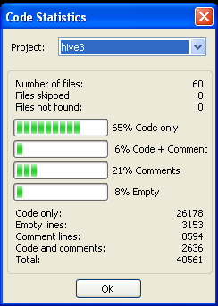
HIVE 3.x BannerCode statistics for HiveWith the inclusion of the phonon-module and some minor fixes and extensions to existing code, the hive 3.x program now counts over 40.000 lines, spread over 60 files. 8% of all lines are blank lines, 71% of all lines contain code, and 21% contain comments, an indication of the extent of the documentation of the code.

The code now provides access to 33 command line options of varying complexity. The simplest options (extracting a geometry, or creating a cif-file) are nearly instantaneous, while more complex options (such as Hirshfeld-I calculations) can take up to several hours.

Also from this point onward, HIVE will require to be linked with a lapack-library during compilation, to allow for the efficient solution of eigenvalue-problems.

Time for a little celebration.

Permanent link to this article: https://dannyvanpoucke.be/hive-40k-en/

Happy Tau-day

June 28th or 6/28 the first three digits of 2\pi aka \tau. In response to the creation of \pi-day (March  14th), June 28th was suggested as \tau-day to celebrate the number representing the ratio between the circumference of a circle and its radius. (And as with most opinions these days there needs to be a lot of controversy and discussion 😎 ) Having no religious preferences for either, I suggest to celebrate both, one with a single pie, and the other with two.

Permanent link to this article: https://dannyvanpoucke.be/happy-tau-day-2015-en/

Phonons: shake those atoms

In physics, a phonon is a collective excitation in a periodic, elastic arrangement of atoms or molecules in condensed matter, like solids and some liquids. Often designated a quasi-particle, it represents an excited state in the quantum mechanical quantization of the modes of vibrations of elastic structures of interacting particles.

— source: wikipedia

Or for simplicity: sound waves; the ordered shaking of atoms or molecules. When you hit a metal bell with a (small) hammer, or make a wineglass sing by rubbing the edges, you experience the vibrations of the object as sound. All objects in nature (going from atoms to stars) can be made to vibrate, and they do this at one or more specific frequencies : their eigenfrequencies or normal frequencies.

Also single molecules, if they are hit (for example by another molecule bumping into them) or receive extra energy in another way, start to vibrate. These vibrations can take many forms (elongating and shortening of bonds, rotating of parts of the molecule with respect to other parts, flip-flopping of loose ends, and so forth) and give a unique signature to the molecule since each of these vibrations (so-called eigen-modes) corresponds with a certain energy given to the molecule. As a result, if you know all the eigen-modes of a molecule, you also know which frequencies of infrared light they should absorb, which is very useful, since in experiment we do not “see” molecules (if we see them at all) as nice ball-and-stick objects.

From the computational point of view, this is not the only reason why in molecular modeling the vibrational frequencies of a system (i.e. the above eigen-modes) are calculated. In addition, they also tell if a system is in its ground state (which is what one is looking for most of the time) or not. Although this tool has wide-spread usage in molecular modeling, it is seldom used in ab initio solid state physics because of the associated computational cost. In addition, because of the finite size of the unit cell, the reciprocal space in which phonons live also has a finite size, in contrast to the single point for a molecule…making life complex. 😎

Continue reading

Permanent link to this article: https://dannyvanpoucke.be/phonons-shake-those-atoms-en/

Tutorial OOP(II): One problem, different possible classes

additional resources
agent paper: Sobkowicz
source-code: AgentTutorials
Arxiv: Full Tutorial

In the previous tutorial, we saw how to tackle an opinion dynamics problem using agents as a class in an Object Oriented Programming (OOP) approach. In many topics of interest in (socio-)physics and chemistry, we deal with a large number of particles, be it electrons, atoms, agents, stars, … These are contained in a superstructure (electrons⇒atom, atoms⇒molecule/solid, agents⇒population, stars⇒galaxy,…) which is generally represented in the code as an array. As we noted in the previous tutorial, there were several variables which were global to the agents, but we implemented them as properties of the agents anyhow. As a result, a significant amount of additional memory needed to be allocated for storing in essence the same data. This was done to prevent the need of having to provide this information at every function call.

Returning to our problem of interest, we now consider two object classes: The TAgent-class and the TPopulation-class. This leads to several possible ways this problem can be implemented.

  1. Array of TAgents: As was done in the previous tutorial, we only make a class of the agents, and put them in an array.
  2. TPopulation of TAgents: In this case we construct a class called TPopulation of which one property is the set of TAgents. The TPopulation-class also contains some of the global variables as properties, and operations on this set are methods of the TPopulation-class.
  3. TPopulation-class without TAgent-class: In this last case, the agents are dissolved, and their properties are stored in array-properties of the TPopulation-class. The methods of the TAgent-class now become methods of the TPopulation-class. And the global variables become additional properties of the TPopulation-class.

Although the true OOP-programmer may only consider the  second option the way to go, we will consider the third option in this tutorial.

Continue reading

Permanent link to this article: https://dannyvanpoucke.be/oop-fortran-tut3-en/