Today was the fifth and last day of our spring school on computational tools for materials science. However, this was no reason to sit back and relax. After having been introduced into VASP (day-2) and ABINIT (day-3) for solids, and into Gaussian (day-4) for molecules, today’s code (CP2K) is one which allows you to study both when focusing on dynamics and solvation.
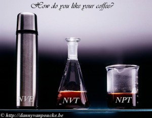
If ensembles were coffee…
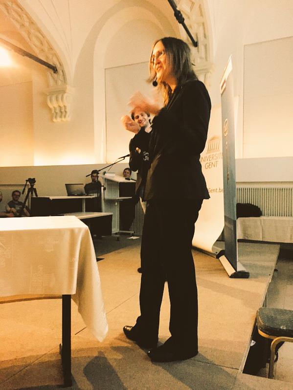
The introduction into the Swiss army knife called CP2K was provided by Dr. Andy Van Yperen-De Deyne. He explained to us the nature of the CP2K code (periodic, tools for solvated molecules, and focus on large/huge systems) and its limitations. In contrast to the codes of the previous days, CP2K uses a double basis set: plane waves where the properties are easiest and most accurate described with plane waves and gaussians where it is the case for gaussians. By means of some typical topics of calculations, Andy explained the basic setup of the input and output files, and warned for the explosive nature of too long time steps in molecular dynamics simulations. The possible ensembles for molecular dynamics (MD) were explained as different ways to store hot coffee. Following our daily routine, this session was followed by a hands-on session.
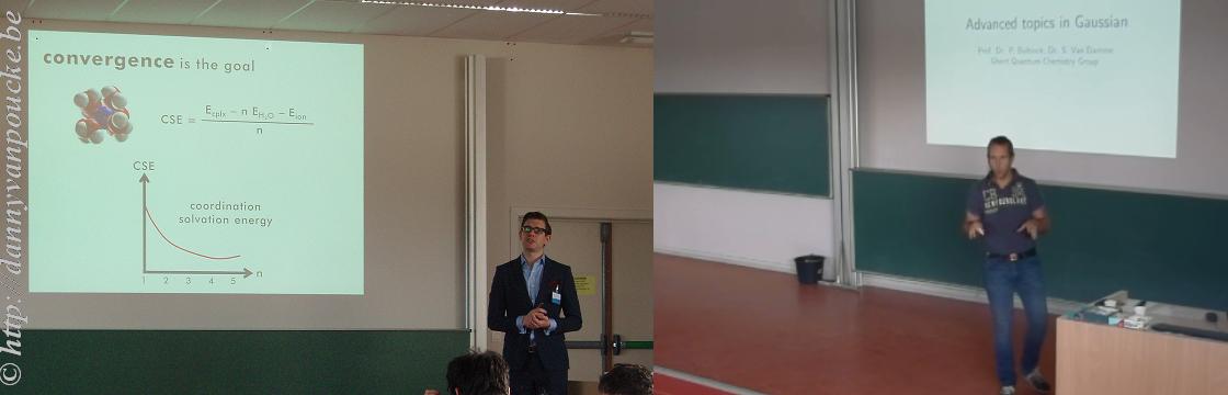
In the afternoon, the advanced session was presented by a triumvirate: Thierry De Meyer, who discussed QM/MM simulations in detail, Dr. Andy Van Yperen-De Deyne, who discused vibrational finger printing and Lennart Joos, who, as the last presenter of the week, showed how different codes can be combined within a single project, each used where they are at the top of their strength, allowing him to unchain his zeolites.
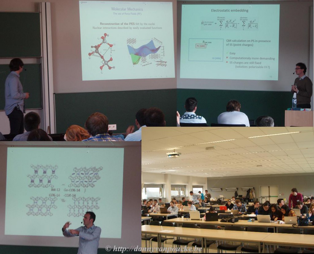
CP2K, all lecturers: Andy Van Yperen-De Deyne (top left), Thierry De Meyer (top right), Lennart Joos (bottom left). All spring school participants hard at work during the hands-on session, even at this last day (bottom right).
The spring school ended with a final hands-on session on CP2K, where the CMM team was present for the last stretch, answering questions and giving final pointers on how to perform simulations, and discussing which code to be most appropriate for each project. At 17h, after my closing remarks, the curtain fell over this spring school on computational tools for materials science. It has been a busy week, and Kurt and I are grateful for the help we got from everyone involved in this spring school, both local and external guests. Tired but happy I look back…and also a little bit forward, hoping and already partially planning a next edition…maybe in two years we will return.
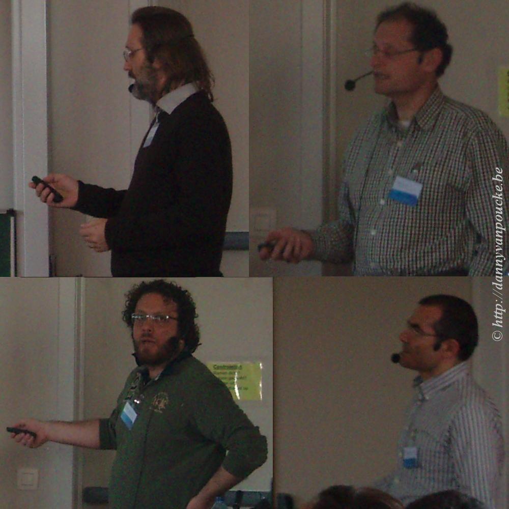
Our external lecturers from the VASP group (Martijn Marsman, top left) and the ABINIT group (Xavier Gonze, top right, Matteo Giantomassi, bottom left, Gian-Marco Rignanese, bottom right)


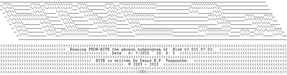
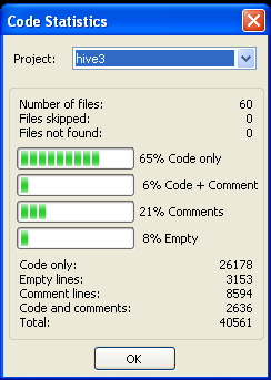 With the inclusion of the phonon-module and some minor fixes and extensions to existing code, the hive 3.x program now counts over 40.000 lines, spread over 60 files. 8% of all lines are blank lines, 71% of all lines contain code, and 21% contain comments, an indication of the extent of the documentation of the code.
 aka
aka  . In response to the creation of