Category: blog

Tutorial OOP(V): Documenting Fortran 2003 Classes

In the previous sessions of this tutorial on Object Oriented Programming in Fortran 2003, the basics of OO programming, including the implementation of constructors and destructors as well as operator overloading were covered. The resulting classes have already become quite extended (cf. github source). Although at this point it is still very clear what each part does and why certain choices were made, memory fades. One year from now, when you revisit your work, this will no longer be the case. Alternately, when sharing code, you don’t want to have to dig through every line of code to figure out how to use it. These are just some of the reasons why code documentation is important. This is a universal habit of programming which should be adopted irrespective of the programming-language and-paradigm, or size of the code base (yes, even small functions should be documented).

In Fortran, comments can be included in a very simple fashion: everything following the “!” symbol (when not used in a string) is considered a comment, and thus ignored by the compiler. This allows for quick and easy documentation of your code, and can be sufficient for single functions. However, when dealing with larger projects retaining a global overview and keeping track of interdependencies becomes harder. This is where automatic documentation generation software comes into play.  These tools parse specifically formatted comments to construct API documentation and user-guides. Over the years, several useful tools have been developed for the Fortran language directly, or as a plugin/extension to a more general tool:

  • ROBODoc : A tool capable of generating documentation (many different formats) for any programming/script language which has comments.  The latest update dates from 2015.
  • Doctran : This tool is specifically aimed at free-format (≥ .f90 ) fortran, and notes explicitly the aim to deal with object oriented f2003. It only generates html documentation, and is currently proprietary with license costs of 30£ per plugin. Latest update 2016.
  • SphinxFortran : This extension to SphinxFortran generates automatic documentation for f90 source (no OO fortran) and generates an html manual. This package is written in python and requires you to construct your config file in python as well.
  • f90doc / f90tohtml : Two tools written in Perl, which transform f90 code into html webpages.
  • FotranDOC : This tool (written in Fortran itself) aims to generate documentation for f95 code, preferably in a single file, in latex. It has a simple GUI interface, and the source of the tool itself is an example of how the fortran code should be documented. How nice is that?
  • FORD : Ford is a documentation tool written in python, aimed at modern fortran (i.e. ≥ f90).
  • Doxygen :  A multi-platform automatic documentation tool developed for C++, but extended to many other languages including fortran. It is very flexible, and easy to use and can produce documentation in html, pdf, man-pages, rtf,… out of the box.

As you can see, there is a lot to choose from, all with their own quirks and features. One unfortunate aspect is the fact that most of these tools use different formatting conventions, so switching from one to the another is not an exercise to perform lightly. In this tutorial, the doxygen tool is used, as it provides a wide range of options, is multi-platform,  supports multiple languages and multiple output formats.

As you might already expect, Object Oriented Fortran (f2003) is a bit more complicated to document than  procedural Fortran, but with some ingenuity doxygen can be made to provide nice documentation even in this case.

1. Configuring Doxygen

Before you can start you will need to install doxygen:

  1. Go the the doxygen-download page and find the distribution which is right for you (Windows-users: there are binary installers, no hassle with compilations 🙂 ).
  2. Follow the installation instructions, also install GraphViz, this will allow you to create nicer graphics using the dot-tool.
  3. Also get a pdf version of the manual (doxygen has a huge number of options)

With a nicely installed doxygen, you can make use of the GUI to setup a configuration suited to your specific needs and generate the documentation for your code automatically. For Object Oriented Fortran there are some specific settings you should consider:
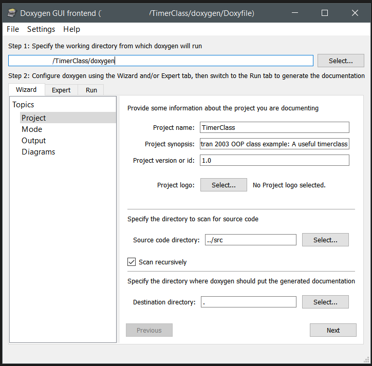
GUI interface of doxygen.

  1.  Wizard tab

    • Project Topic : Fill out the different fields. In a multi-file project, with source stored in a folder structure, don’t forget to select the tick-box “Scan recursively” .
    • Mode Topic : Select “Optimize for Fortran output”.
    • Output Topic : Select one or more output formats you wish to generate: html, Latex (pdf), map-pages, RTF, and XML
    • Diagrams Topic: Select which types of diagrams you want to generate.
  2. Expert tab

    (Provides access each single configuration option to set in doxygen, so I will only highlight a few. Look through them to get a better idea of the capabilities of doxygen.)

    • Project Topic :
      • EXTENSION_MAPPING: You will have to tell doxygen which fortran extensions you are using by adding them, and identifying it as free format fortran: e.g. f03=FortranFree (If you are also including text-files to provide additional documentation, it is best to add them here as well as free format fortran).
    • Build Topic:
      • CASE_SENSE_NAMES: Even though Fortran itself is not case sensitive, it may be nice to keep the type of casing you use in your code in your documentation. Note, however, that even though the output may have upper-case names, the documentation itself will require lower-case names in references.
    • Messages Topic:
      • WARN_NO_PARAMDOC: Throw a warning if documentation is missing for a function variable. This is useful to make sure you have a complete documentation.
    • Source Browser Topic:
      • SOURCE_BROWSER: Complete source files are included in the documentation.
      • INLINE_SOURCES: Place the source body with each function directly in the documentation.
    • HTML Topic:
      • FORMULA_FONTSIZE: The fontsize used for generated formulas. If 10 pts is too small to get a nice effect of formulas embedded in text.
    • Dot Topic:
      • HAVE_DOT & DOT_PATH: If you installed GraphViz
      • DOT_GRAPH_MAX_NODES: Maximum number of nodes to draw in a relation graph. In case of larger projects, 50 may be too small.
      • CALL_GRAPH & CALLER_GRAPH: Types of relation graphs to include.
  3. Run tab

    • Press “Run doxygen” and watch how your documentation is being generated. For larger projects this may take some time. Fortunately, graphics are not generated anew if they are present from a previous run, speeding things up. (NOTE: If you want to generate new graphics (and equations with larger font size), make sure to delete the old versions first.) Any warnings and errors are also shown in the main window.
    • Once doxygen was run successfully, pressing the button “Show HTML output” will open a browser and take you to the HTML version of the documentation.


Once you have a working configuration for doxygen, you can save this for later use. Doxygen allows you to load an old configuration file and run immediately. The configuration file for the Timer-class project is included in the docs folder, together with the pdf-latex version of the generated documentation.  Doxygen generates all latex files required for generating the pdf. To generate the actual pdf, a make.bat file needs to be run (i.e. double-click the file, and watch it run) in a Windows environment.

2. Documenting Fortran (procedural)

Let us start with some basics for documenting Fortran code in a way suitable for doxygen. Since doxygen has a very extensive set of options and features, not all of them can be covered. However, the manual of more than 300 pages provides all the information you may need.

With doxygen, you are able to document more or less any part of your code: entire files, modules, functions or variables. In each case, a similar approach can be taken. Let’s consider the documentation of the TimeClass module:

  1. !++++++++++++++++++++++++++++++++++++++++++++++++++++++++++++++++++++++++
  2. !> \brief The <b>TimeClass module</b> contains the
  3. !! \link ttime TTime class\endlink used by the
  4. !! \link timerclass::ttimer TTimer class\endlink for practical timing.
  5. !!
  6. !! @author  Dr. Dr. Danny E. P. Vanpoucke
  7. !! @version 2.0-3  (upgrades deprecated timing module)
  8. !! @date    19-03-2020
  9. !! @copyright https://dannyvanpoucke.be
  10. !!
  11. !! @warning Internally, Julian Day Numbers are used to compare dates. As a
  12. !! result, *negative* dates are not accepted. If such dates are created
  13. !! (*e.g.*, due to a subtraction), then the date is set to zero.
  14. !!
  15. !! This module makes use of:
  16. !! - nothing; this module is fully independent
  17. !<-----------------------------------------------------------------------
  18. module TimeClass
  19.     implicit none
  20.     private

The documentation is placed in a standard single or multi-line fortran comment.  In case of multi-line documentation, I have the personal habit turning it into a kind of banner starting with a “!+++++++++” line and closing with a “!<——————-” line.  Such choices are your own, and are not necessary for doxygen documentation. For doxygen, a multi-line documentation block starts with “!>” and ends with “!<“ . The documentation lines in between can be indicated with “!!”. This is specifically for fortran documentation in doxygen. C/C++ and other languages will have slightly different conventions, related to their comment section conventions.

In the block above, you immediately see certain words are preceded by an “@”-symbol or a “\”, this indicates these are special keywords. Both the “@” and “\” can be used interchangeably for most keywords, the preference is again personal taste.  Furthermore, doxygen supports both html and markdown notation for formatting, providing a lot of flexibility. The multi-line documentation is placed before the object being documented (here an entire module).

Some keywords:

  • \brief : Here you can place a short description of the object. This description is shown in parts of the documentation that  provide an overview. Note that this is also the first part of the full documentation of the object itself. After a blank line, the \details(this keyword does not need to provided explicitly) section starts, providing further details on the object. This information is only visible in the documentation of the object itself.
  • \link … \endlink, or \ref : These are two option to build links between parts of your documentation. You can either use \ref nameobject or \link nameobject FormattedNameObject \endlink. Note that for fortran, doxygen uses an all non-capitalized namespace, so YourObject needs to be referenced as \ref yourobject or you will end up with an error and a missing link. So if you want your documentation to show YourObject as a link instead of yourobject, you can use the \link … \endlink construction.
  • “::”  : Referring to an element of an object can be done by linking the element and the object via two colons:  object::element . Here it is important to remember that your module is an object, so linking to an element of a module from outside that module requires you to refer to it in this way.
  • @author : Provide information on the author.
  • @version : Provide version information.
  • @date : Provide information on the date.
  • @copyright : Provide information on the copyright.
  • @warning : Provides a highlighted section with warning information for the user of your code (e.g., function kills the program when something goes wrong).
  • @todo[not shown] If you still have some things to do with regard to this object you can use this keyword. More interestingly, doxygen will also create a page where all to-do’s of the entire project are gathered, and link back to the specific code fragments.


  1. !++++++++++++++++++++++++++++++++++++++++++++++
  2. !>\brief Function to subtract two \link ttime TTime\endlink instance
  3. !! via the "-" operator. This is the function
  4. !! performing the actual operator overloading.
  5. !!
  6. !! \b usage:
  7. !! \code{.f03}
  8. !! Total = this - that
  9. !! \endcode
  10. !! This line also calls the \link copy assignment operator\endlink.
  11. !!
  12. !! \note The result should remain a positive number.
  13. !!
  14. !! @param[in] this The \link ttime TTime\endlink instance before
  15. !!                 the "-" operator.
  16. !! @param[in] that The \link ttime TTime\endlink instance after
  17. !!                 the "-" operator.
  18. !! \return Total The \link ttime TTime\endlink instance representing
  19. !!               the difference.
  20. !<---------------------------------------------
  21.     pure function subtract(this,that) Result(Total)
  22.         class(TTime), intent(in) :: this, that
  23.         Type(TTime) :: total

When documenting functions and subroutines there are some addition must-have keywords.

  • @param[in] , @param[out] ,or@param[in,out] : Provide a description for each of the function parameters, including their  intent: “in”, “out”, or “in,out” (note the comma!).
  • \return : Provides information on the return value of the function.
  • \b, \i : The next word is bold or italic
  • \n : Start a newline, without starting a new paragraph.
  • \note : Add a special note in your documentation. This section will be high lighted in a fashion similar to @warning.
  • \code{.f03}…\endcode :  This environment allows you to have syntax highlighted code in your documentation. The language can be indicated via the “extension” typical for said language. In this case: fortran-2003.
  • \f$ … \f$, or \f[ … \f] : Sometimes equations are just that much easier to convey your message. Doxygen also supports latex formatting for equations. These tags can be used to enter a latex $…$ or \[ \] math environments. The equations are transformed into small png images upon documentation generation, to be included in the html of your documentation. There are two important aspects to consider when using this option:
    1. Font size of the equation: Check if this is sufficient and don’t be afraid to change the font size to improve readability.
    2. Compilation is not halted upon an error: If the latex compiler encounters an error in your formula it just tries to continue. In case of failure, the end result may be missing or wrong. Debugging latex equations in doxygen documentation can be quite challenging as a result. So if you are using large complex equations, it may be advised to run them in a pure latex environment, and only past them in the documentation once you are satisfied with the result.


3. Documenting Fortran Classes

With the knowledge of the previous section, it is relatively easy to document most fortran code. Also the type of object orientation available in fortran 95, in which a fortran module is refurbished as a class. True fortran classes in contrast tend to give a few unexpected issues to deal with. Lets have a look at the documentation of the TTime class of the TimeClass module:

  1. !+++++++++++++++++++++++++++++++++++++++
  2. !> @class ttime
  3. !! \brief The TTime class contains all time functionality
  4. !! with regard to a single time stamp.
  5. !<-------------------------------------
  6.     type, public :: TTime
  7.       private
  8.         integer :: year    !< @private The year
  9.         integer :: month   !< @private The month (as integer).
  10.         ...
  11.     contains
  12.       private
  13.         procedure, pass(this),public :: SetTime       !<          @copydoc timeclass::settime
  14.         procedure, pass(this)        :: CalculateJDN  !< @private @copydoc timeclass::calculatejdn
  15.         procedure, pass(this)        :: SetJDN        !< @private @copydoc timeclass::setjdn
  16.         ...
  17.         procedure, pass(this)        :: copy          !< @private @copydoc timeclass::copy
  18.         ...
  19.         generic, public :: assignment(=) => copy      !<          @copydoc timeclass::copy
  20.         !> @{ @protected
  21.         final :: destructor !< @copydoc timeclass::destructor
  22.         !> @}
  23.     end type TTime
  24.  
  25.     ! This is the only way a constructor can be created,
  26.     ! as no "initial" exists, emulates the C++ constructor behavior
  27.     interface TTime
  28.         module procedure constructor
  29.     end interface TTime

To make sure doxygen generates a class-like documentation for our fortran class, it needs to be told it is a class. This can be done by documenting the class itself and using the keyword @class nameclass, with nameclass the name doxygen will use for this class (so you can choose something different from the actual class name). Unfortunately, doxygen will call this a “module” in the documentation (just poor luck in nomenclature). On the module page for the ttime class a listing is provided of all elements given in the class definition. The documentation added to each member (e.g.,:

  1. integer :: year !< @private The year

is shown as “\brief” documentation. By default all members of our function are considered as public. Adding the @private, @public, or @protected keyword instructs doxygen explicitly to consider these members as private, public or protected. (I used protected in the ttime code not as it should be used in fortran, but as a means of indicating the special status of the final subroutine (i.e. protected in a C++ way).)

However, there seems to be something strange going on. When following the links in the documentation, we do not end up with the documentation provided for the functions/subroutines in the body of our timeclass module. Doxygen seems to consider these two distinct things. The easiest way to link the correct information is by using the keyword @copydoc functionreference . The documentation is (according to doxygen) still for two distinctly different objects, however, this time they have the exact same documentation (unless you add more text on the member documentation line). In this context, it interesting to know there is also @copybrief and @copydetails which can be used to only copy the brief/details section.

In this example, the constructor interface is not documented, as this created confusion in the final  documentation since doxygen created a second ttime module/object linked to this interface. However, not documenting this specific instance of the constructor does not create such a large issue, as the module(the fortran module) function itself is documented already.

Conclusion

Documenting fortran classes can be done quite nicely with doxygen. It provides various modes of output: from a fully working website with in-site search engine to a hyperlinked pdf or RTF document. The flexibility and large number of options may be a bit daunting at first, but you can start simple, and work your way up.

As Fortran is supported as an extension, you will need to play around with the various options to find which combination gives the effect you intended. This is an aspect present in all automated code documentation generation tools, since object oriented Fortran is not that widely used. Nonetheless, doxygen provides a very powerful tool worth your time and effort.

PS:

SBDD 25 (aka the COVID19 edition)

Last Wednesday, the 25th edition of the Hasselt Diamond workshop started. The central topic of this celebratory edition was focused on surfaces, perfectly suited to present some of my more recent diamond based work.[1][2] Just as the previous years, the program was packed with interesting talks on anything diamond. Phosphorous doped diamond seemed to be the “new thing” this year, but I could be biased, as I was speaking on phosphorous adsorption myself. Due to a cancellation, I found myself being asked on Monday afternoon to present my work as a talk 😎 , on Wednesday morning 😯 . Because I had been a bit too ambitious in my conference abstract, this talk ended up being nicely complementary to my poster.

Poster SBDD 25 conference, Hasselt 2020

Unfortunately, this celebratory edition also fell victim to the COVID-19 crisis. In addition to being the most popular conversation topic—a close second to diamond research—, it also had a very real impact on the conference itself. The COVID-19 crisis resulted in a drop of attendance from 238 people in 2019 to 143 this year.  In addition, the quickly changing situation worldwide lead to last minute cancellations due to travel restrictions. On Thursday evening, the conference site went into lock down. Furthermore, that evening, the Belgian federal government also decided that schools and higher education should be closed, as well as pubs and restaurants, until April 3rd. There was also the urgent request for people to work from home as much as possible. (Consider this a good example of acting NOW aimed at saving people.)

Consider this computational scientist in lock down in his home lab until further notice.

Review of 2019

Happy New Year

2019 has come and gone. 2020 eagerly awaits getting acquainted. But first we look back one last time, trying to turn this into a old tradition. What have I done during the last year of some academic merit.

Publications: +3 (and currently +5 submitted)


Completed refereeing tasks: +9

  • Applied Physics Letters
  • Journal of Physics Communication
  • Super Conducting Science and Technology
  • Crystals
  • Journal of Physics: Condensed Matter (2x)
  • Diamond and Related Materials (3x)


Conferences & workshops: +7 (Attended) 

  • Consortium meeting D-NL-HIT, Hochschule Niederrhein, Krefeld, Germany, September 19th 2019
  • Workshop: Coatings Technology & Application of Machine Learning, Hochschule Niederrhein, Krefeld, Germany, September 2nd-6th , 2019
  • Summer School: “Let’s Talk Science”, Antwerp, Belgium, July 2nd, 2019 [invited plenary talk]
  • Summer School on Data Science, Maastricht University, The Netherlands, June 26th-28th,  2019
  • VSC-user day, Brussels, Belgium, June 4th, 2019 [poster presentation]
  • Belgian Physical Society annual meeting 2019, ULB, Brussels, May 22nd, 2019 [poster presentation]
  • SBDD XXIV, Hasselt University, Belgium, March 13th-15th, 2019


Science Communication Events: +3  

  • Casting Keynotes TEDxUHasselt:”The Virtual Lab”, November 26th, 2019 [first prize, TEDx talk 2020]
  • Summer School: “Let’s Talk Science”, Antwerp, Belgium, July 2nd, 2019 [invited plenary talk]
  • Universiteit van Vlaanderen: “Kan jij met je computer een snellere smartphone ontwikkelen”, February 19th, 2019 [Live presentation at UvV, Online April 1st]


Research Stay: +1           With Prof. Klauss-Uwe Koch, Westfälishe Hochschule, Recklinghausen, Germany, July 29th – August 2nd, 2019

PhD-students: +1             Guillaume Emerick (September 2019-August 2023,PhD student UHasselt-UNamur Project, Belgium, Awarded grant for this project)

Bachelor-students: +1   Siebe Frederix (3rd Bach. Phys., Project: Atoms in Molecules based on force partitioning)

Positions: +1                         Started working on Machine Learning at AMIBM of Maastricht University


Current size of HIVE:

  • Finally started a public version of HIVE at github: HIVE 4.x   (3.5K lines, 6 commands available)
  • 60K lines of program (code: 70 %)
  • ~90 files
  • 49 (command line) options

Hive-STM program:

And now, upward and onward, a new year, a fresh start.

Parallel Python?

As part of my machine learning research at AMIBM, I recently ran into the following challenge: “Is it possible to do parallel computation using python.” It sent me on a rather long and arduous journey, with the final answer being something like: “very reluctantly“.

Python was designed with one specific goal in mind; make it easy to implement small test programs to see if an idea is worth pursuing. This gave rise to a scripting language with a lot of flexibility, but also with significant limitations, most of which the “intended” user would never meet. However, as a consequence of its success, many are using it going far beyond this original scope (yours truly as well 🙂 ).

Python offers various libraries to parallelize your scripts…most of them wrappers adding minor additional functionality. However, digging down to the bottom one generally ends up at one of the following two libraries: the threading module and the multiprocessing module.

Of course, as with many things python, there is a huge amount of tutorials available with many of great quality.

import threading

Programmers experienced in a programming language such as C/C++, Pascal, or Fortran, may be familiar with the concept of multi-threading. With multi-threading, a CPU allows a program to distribute its work over multiple program-threads which can be performed in parallel by the different cores of the CPU (or while a core is idle, e.g., since a thread is waiting for data to be fetched).  One of the most famous API’s for writing multi-threaded applications is OpenMP. In the past I used it to parallelize my Hirshfeld-I implementation and the phonon-module of HIVE.

For Python, there is no implementation of the OpenMP API, instead there is the threading module. This provides access to the creation of multiple threads, each able to perform their own tasks while sharing data-objects. Unfortunately, python has also the Global Interpreter Lock, GIL for short, which allows only a single thread to access the interpreter at a time. This effectively reduces thread-based parallelization to a complex way of running a code in a serial way.

For more information on “multi-threading” in python, you can look into this tutorial.

import multiprocessing

In addition to the threading module, there is also the multiprocessing module. This module side-steps the GIL by creating multiple processes, each having its own interpreter. This however comes at a cost. Firstly, there is a significant computational cost starting the different processes. Secondly, objects are not shared between processes, so additional work is needed to collect and share data.

Using the “Pool” class, things are somewhat simplified, as can be seen in the code-fragment below.  With the pool class one creates a set of threads/processes available for your program. Then through the function apply_async function it is possible to run processes in parallel. (Note that you need to use the “async” version of the function, as otherwise you end up with running things serial …again)

  1. import multiprocessing as mp
  2.  
  3. def doOneRun(id:int): #trivial function to run in parallel
  4. return id**3
  5.  
  6.  
  7.  
  8. num_workers=10 #number of processes
  9. NRuns=1000 #number of runs of the function doOneRun
  10.  
  11. pool=mp.Pool(processes=num_workers) # create a pool of processes
  12. drones=[pool.apply_async(doOneRun, args=nr) for nr in range(NRuns)] #and run things in parallel
  13.  
  14. for drone in drones: #and collect the data
  15. Results.collectData(drone.get()) #Results.collectData is a function you write to recombine the separate results into a single result and is not given here.
  16.  
  17. pool.close() #close the pool...no new tasks can be run on any of the processes
  18. pool.join() #collapse all threads back into the main thread


how many cores does my computer have?

If you are used to HPC applications, you always want to get as much out of your machine as possible. With regard to parallelization this often means making sure no CPU cycle is left unused. In the example above we manually selected the number of processes to spawn. However, would it not be nice if the program itself could just set this value to be equal to the number of physical cores accessible?

Python has a large number of functions claiming to do just that. A few of them are given below.

  •  multiprocessing.cpu_count(): returns the number of logical cores it can find. So if you have a modern machine with hyper-threading technology, this will return a multiple of the number of physical cores (and you will be over-subscribing your CPU.
  • os.cpu_count(): same as multiprocessing.cpu_count().
  • psutil.cpu_count(logical=False): This implementation gives the same default behavior, however, the parameter logical allows for this function to return the correct number of cores in a single CPU. Indeed a single CPU. HPC architectures which contain multiples CPUs per node will again return an incorrect number, as the implementation makes use of a python “set”, and as such doesn’t increment for the same index core on a different CPU.

In conclusion, there seems to be no simple way to obtain the correct number of physical cores using python, and one is forced to provide this number manually. (If you do have knowledge of such a function which works in both windows and unix environments and both desktop and HPC architectures feel free to let me know in the comments.)

All in all, it is technically possible to run code in parallel using python, but you have to deal with a lot of python quirks such as GIL.

Casting Keynotes: The Virtual Lab

Last Tuesday? I had the pleasure of competing in the casting keynotes competition of the TEDx UHasselt chapter. An evening filled with interesting talks on subjects ranging from the FAIR principles of open-data (by Liebet Peeters)  to the duty not stay silent in the face of “bad ideas” and leading a life of purpose. An interesting presentation was the one by Ann Bessemans on visual prosody to improve reading skills in young children as well as reading experience, more specifically the transfer of non-literal-content, for non-native speakers. There was also time for some humor, with the dangerous life of Tim Biesmans, who suffers from peanut-allergies. For him, death lurks around every corner, even in a first-date’s kiss. During my talk, I traced the evolution of computational research as the third paradigm of scientific discovery, showing you can find computational research in every field, and why it is evolving at its break-neck speed.

During the event, both the public and a jury voted on the best presentation, which would then have to present at the TEDx UHasselt in 2020.

And the Winner is …drum roll… Danny Vanpoucke!

So this story will continue during the 2020 TEDx event at UHasselt, and I hope to see you there 🙂

Casting Keynotes

top: Full action shots of my presentation. Moore’s Law as driving force behind computational research, and pondering the meaning of Artificial Intelligence. Bottom: Yes, I won 🙂


Tutorial OOP(IV) : Operator and Assignment Overloading

In the previous tutorial, we created a constructor and destructor for our TTimer class.  Next, we extend our class with overloaded operators. Depending on the type of object your class represents, you may want to define an addition/subtraction/multiplication/… operator. In addition, the assignment operator deserves some extra attention as you may want to have a clear control over this operation  (e.g.deep copy vs shallow copy). The full source of this tutorial and the previous, can be downloaded from my github-page.

Let us start with the latter: the assignment operator. As with all other operators, it is possible to overload the assignment operator in modern fortran.

1. Assignment (=) operator overloading

When dealing with objects and classes—or extended data-structures in general—, their properties often are (implicit) pointers to the actual data-structure. This brings an interesting source of possible bugs due to shallow copies being made while deep copies are expected (although the problem may be less pronounced in Fortran than it is in Python).

In a fortran object, the assignment of a pointer component (i.e., an explicit pointer variable, or a component which is an object itself) happens via a shallow copy (or pointer assignment). In contrast, for an allocatable component, the assignment operation performs by default a deep copy (i.e., space is allocated, and values are copied). Shallow copies are very useful with regard to quickly creating new handles to the same data-structure. However, if you want to make a true copy, which you can modify without changing the original, then a deep copy is what you want. By implementing assignment overloading for your own classes, you have more control over the actual copying process, and you can make sure you are creating deep copies if those are preferred.

The implementation of overloading for the assignment operator is not too complicated. It requires two lines in your class definition:

type, public :: TTimer
        private
        ...
    contains
        private
        procedure, pass(this) :: Copy                   !< Make a copy of a timer object
        generic, public       :: assignment(=) => Copy  !< This is how copy is used.
        ...
end type TTimer

First, you need to define a class method which performs a copy-operation—which in a fit or original though we decided to call “copy” ;-).  As you can see this function is private, so it will not be accessible to the user of your class via a call like :

call MyTimer%Copy()

Secondly, you link this class method via the “=>” to the assignment-operator.  It is a generic interface, which means the assignment operator could be linked to different functions, of which the relevant one will be determined and used during run-time. This generic is also public  (otherwise you would not be able to use it).

The implementation of the class method follows the standard rules of any class method and could look like

pure subroutine Copy(this,from)
        class(TTimer), intent(inout) :: this
        class(TTimer), intent(in) :: from

    this%firstProperty = from%firstProperty
    ...
    !make explicit copies of all properties and components
    ...

end subroutine Copy

The “this” object which we passed to our class method is the object on the left side of the assignment operator, while the “from” object is the one on the right side. Note that both objects are defined as “class” and not as “type”. Within the body of this method you are in charge of copying the data from the “from”-object to the “this”-object, giving you control over deep/shallow copying.

In practice the overloaded operator is used as:

type(TTimer):: TimerThis, TimerFrom

TimerFrom = TTimer() ! initialization of the timers
TimerThis = TTimer() ! (cf., previous tutorial on constructors and destructors)
... 
! do stuff with TimerFrom
...
TimerThis = TimerFrom ! although you type "=", the overloading causes this to be implemented as-if you wrote
                      ! call TimerThis%copy(TimerFrom)

2. Operator (+,-,*,/,…) overloading

Just as you can overload the assignment operator above, you can also overload all other fortran operators. However, be careful to keep things intuitive.  For example, an addition operation on our TTimer class is strange. What would it mean to add one timer to another? How would you subtract one chronometer from another? In contrast, inside our TTimer class we have a list of TTime objects which can be used to represent a date and time, as-well-as a time interval.[1]  For the remainder of this tutorial, we will assume the TTime class only represents time-intervals. For such a class, it makes sense to be able to add and subtract time intervals.

Let us start with the basic definition of our TTime-class:

type, public :: TTime
  private
   ...
   ! the properties of the TTime class
   ...
contains
  private
   ...
   ! the methods of the TTime class
   ... 
   procedure, pass(this)        :: copy          ! Copy content from other TTime instance,  
                                                 ! private, accessed via the assignment statement
   procedure, pass(this)        :: add           ! Add two TTime instances.
   procedure, pass(this)        :: subtract      ! subtract two TTime instances.
   generic, public :: assignment(=) => copy      ! This is how copy is used.
   generic, public :: operator(+)   => add       ! This is how add is used.
   generic, public :: operator(-)   => subtract  ! This is how subtract is used.
   final :: destructor
end type TTime

interface TTime
   module procedure constructor
end interface TTime

The TTime class has a constructor and destructor, implemented as we discussed before. The assignment operator is over-loaded as well. The overloading of the “+” and “” operator follows the same setup as for the assignment operator. First, you define a class method where you will implement the addition or subtraction. Second, you link this class method to the operator as a generic. The main difference with overloading the assignment operator is that you need to use the keyword operator instead of assignment, during the second step. The class methods are private, while the generic link is public. The only thing left to do is to implement the class methods. In case of operator overloading, the class methods are functions.

pure function add(this,that) Result(Total)
     class(TTime), intent(in) :: this, that
     Type(TTime) :: total

total = TTime()
...
! implementation of the addition of the properties of 
! this to the properties of that, and storing them in 
! Total
! e.g.: Total%seconds = this%seconds + that%seconds        
...
end function add

The returned object need to be defined as a type, and the further implementation of the function follows the standard fortran rules. It is important to note that for a function-header like this one, the object to the left of the operator will be the one calling the overloaded operator function, so:

Total = this + that

and not

Total = that + this

This may not seem this important, as we are adding two objects of the same class, but that is not necessarily always the case. Imagine that you want to overload the multiplication operator, such that you could multiply your time-interval with any possible real value. On paper

Δt * 3.5 = 3.5 * Δt

but for the compiler in the left product “this” would be a TTime object and “that” would be a real, while in the right product “this” is the real, and “that” is the TTime object. To deal with such a situation, you need to implement two class methods, which in practice only differ in their header:

pure function MultLeft(this,that) Result(Total) 
    class(TTime), intent(in) :: this
    real, intent(in) :: that 
    Type(TTime) :: total

and

pure function MultRight(that, this) Result(Total) 
    class(TTime), intent(in) :: this
    real, intent(in) :: that 
    Type(TTime) :: total

In the class definition both functions are linked to the operator as

procedure, pass(this) ::  MultLeft
procedure, pass(this) ::  MultRight
generic, public :: operator(*) => MultLeft, MultRight

With this in mind, we could also expand our implementation of the “+” and “” operator, by adding functionality that allows for the addition and subtraction of reals representing time-intervals. Also here, the left and right versions would need to be implemented.

As you can see, modern object oriented fortran provides you all the tools you need to create powerful classes capable of operator overloading using simple and straightforward implementations.

In our next Tutorial, we’ll look into data-hiding and private/public options in fortran classes.


[1] You could argue that this is not an ideal choice and that it would be better to keep these two concepts ( absolute and relative time) separate through the use of different classes. 

Tutorial OOP(III): Constructors and Destructors

In this tutorial on Object Oriented Programming in Fortran 2003, we are going to discuss how to create constructors and destructors for a Fortran class. During this tutorial, I assume that you know how to create a new project and what a class looks like in Fortran 2003.  This tutorial is build around a TimerClass, which I wrote as an upgrade for my initial timing module in HIVE-tools. The full source of this TimerClass can be found and downloaded from github.

Where the former two tutorials were aimed at translating a scientific model into classes within the confines of the Fortran programming language, this tutorial is aimed at consolidating a class using good practices: The creation a constructor and destructor. As the destructor in Fortran classes is most straight forward of the two, we’ll start with it.

1. The destructor.

A destructor is a method (i.e., a class subroutine) which is automatically invoked when the object is destroyed (e.g., by going out of scope).  In case of a Fortran class, this task is performed by the class-method(s) indicated as  final procedure. Hence such methods are also sometimes referred to as finalizers. Although in some languages destructors and finalizers are two distinctly different features (finalizers are then often linked to garbage collecting), within the Fortran context I consider them the same.

Within the definition of our TTimerClass the destructor is implemented as:

  1. module TimerClass
  2. implicit none
  3.  
  4.     type, public :: TTimer
  5.       private
  6.       ! here come the properties
  7.     contains
  8.       private
  9.       ! here come the methods
  10.       final :: destructor
  11.     end type TTimer
  12.    
  13. contains
  14.  
  15.     subroutine destructor(this)
  16.     Type(TTimer) :: this
  17.     ! Do whatever needs doing in the destructor
  18.     end subroutine destructor
  19.    
  20. end module TimerClass

In contrast to a normal class-method, the destructor is called using the final keyword, instead of the usual procedure keyword. This method is private, as it is not intended to be used by the user anyway, only by the compiler upon cleanup of the instance of the class (i.e., the object). Furthermore, although defined as part of the class, a final subroutine is not type-bound, and can thus not be accessed through the type.

The destructor subroutine itself is a normal Fortran subroutine. There is, however, one small difference with a usual class-method, the parameter referring to the object (c.q. “this“) is indicated as a TYPE and not as a CLASS. This is because the destructor is only applicable to properties belonging to this “class” (Note that final subroutines are not inherited by the child-class). For a child-class (also called a derived class), the destructor of the child-class should deal with all the additional properties of the child-class, while the destructor of the parent-class is called to deal with its respective properties. In practice, the destructor of the child-class is called first, after which the destructor of the parent class is called (and recursively further along the class its family tree.)

So what do you put in such a destructor? Anything that needs to be done to allow the object to be gracefully terminated. Most obviously: deallocation of allocatable arrays, pointer components, closing file handles,…

2. The constructor.

Where other programming  languages may provide an initialization section or access to a key-worded constructor. Although Fortran allows for variables to be initialized upon definition, there is no constructor keyword available to be used in its classes. Of course, this does not prevent you from adding an “init()” subroutine which the user should call once the new object is allocated. You could even use a private Boolean property (initialized old style)  to keep track of the fact that an object was initialized when entering any of its methods, and if not, call the init() function there and then. There are many ways to deal with the initialization of a new object.  Furthermore, different approaches also put the burden of doing things right either with the programmer developing the class, or the user, applying the class and creating objects.

Here, I want to present an approach which allows you to present a clear set-up of your class and which resembles the instance creation approach also seen in other languages (and which implicitly shows the “pointer”-nature of objects ):

NewObject = TClass()

In case of our TTimer class this will look like:

Type(TTimer) :: MyTimer

MyTimer = TTimer()

This means we need to have a function with the exact same name as our class (cf., above), which is achieved through the use of an interface to a module procedure.  Just giving this name to the constructor function itself will cause your compiler to complain (“Name ttimer at (1)  is already defined as a generic interface“).  By using a different name for the  function, and wrapping it in an interface, this issue is avoided.

  1. module Timerclass
  2.     implicit none
  3.  
  4.  
  5.     type, public :: TTimer
  6.         private
  7.     ...
  8.     contains
  9.         private
  10.         ...
  11.     end type TTimer
  12.    
  13.     interface TTimer
  14.         module procedure Constructor
  15.     end interface TTimer
  16.  
  17. contains
  18. function Constructor() Result(Timer)
  19.     type(TTimer) :: Timer
  20.    
  21.     !initialize variables directly
  22.     Timer%x=...
  23.     ! or through method calls
  24.     call Timer%setTime(now)
  25.     ...
  26.  
  27. end function Constructor
  28.  
  29. end module TimerClass

Note that the constructor function is not part of the class definition, and as such the object is not passed to the constructor function. In addition, the Timer object being created is defined as a Type(TTimer) not Class(TTimer), also because this function is not part of the class definition.

That is all there is to it. Simple and elegant.

In our next Tutorial, we’ll have a look at operator and assignment overloading. Combined with a constructor and destructor as presented here, you are able to create powerful and intuitive classes (even in Fortran).

Workshop Machine Learning for Coatings: ML in the Lab (day 5)

On the fifth and final day of the workshop we return to the lab. Our task as a group: optimize our raspberry pink lacquer with regard to hardness, glossiness and chemical resistance.

The four cans of base material made during day 1 of the workshop were mixed to make sure we were all using the same base material (there are already sufficient noise introducing variables present, so any that can be eliminated should be.). Next, each team got a set of recipes generated with the ML algorithm to create. The idea was to parallelise the human part of the process. This would actually also have made for a very interesting exercise to perform in a computer science program. It showed perfectly how bottlenecks are formed and what impact is of serial sections and access/distribution of resources (or is this just in my mind? 😎  ).  After a first round of samples, we already tried to improve the performance of our unit by starting the preparation of the next batch (prefetching 😉 ) while the results of the previous samples were entered into the ML algorithm, and that was run.

At the end of two update rounds, we discussed the results, there were already some clear improvements visible, but a few more rounds would have been needed to get to the best situation. A very interesting aspect to notice during such an exercise, is the difference in the concept of accuracy for the experimental side and the computational side of the story. While the computer easily spits out values in grams with 10 significant digits, at the experimental side of the story it was already extremely hard to get the same amounts with an accuracy of 0.02 gram (the present air currents give larger changes on the scale).

This workshop was a very satisfying experience. I believe I learned most with regard to Machine Learning from the unintentional observation in the lab. Thank you Christian and Kevin!  


Workshop Machine Learning for Coatings: Stochos and DGCN (day 4)

Day 4 of the workshop is again a machine learning centered day. Today we were introduced into the world of Gaussian Processes, and ML approach which is rooted in statistics and models data by looking at the averages of a distribution of functions…it is a function of functions. In contrast to most other ML approaches it is also very well suited for small data sets, which is why I had my eye on them already for quite some time. However, Gaussian Processes are not perfect and interestingly enough, their drawbacks and benefits seem quite complementary with the benefits and drawbacks to neural networks. Deep Gaussian Covariance Networks (DGCN) find their origin in this observation, and were designed with the idea of compensating the drawbacks of both approaches by combining them. The resulting approach is rather powerful and in contrast to any other ML approach: it does not have any hyper-parameter!!

Tomorrow, during the last day of the workshop, we will be using this DGCN to optimize our raspberry pink lacquers.

Book Chapter on Zeolites: Now Open Access

Zeolites and Metal-Organic Frameworks

Zeolites and Metal-Organic Frameworks

Some good new news: The book on zeolites and porous frameworks for which I wrote a chapter on modeling with Bartlomiej Szyja has become open access and can be found here.