Category: blog

New year’s resolution

A new year, a new beginning.

For most people this is a time of making promises, starting new habits or stopping old ones. In general, I forgo making such promises, as I know they turn out idle in a mere few weeks without external stimulus or any real driving force.

In spite of this, I do have a new years resolution for this year: I am going to study machine learning and use it for any suitable application I can get my hands on (which will mainly be materials science, but one never knows).  I already have a few projects in mind, which should help me stay focused and on track. With some luck, you will be reading about them here on this blog. With some more luck, they may even end up being part of an actual scientific publication.

But first things first, learn the basics (beyond hear-say messages of how excellent and world improving AI is/will be). What are the different types of machine learning available, is it all black box or do you actually have some control over things. Is it a kind of magic? What’s up with all these frameworks (isn’t there anyone left who can program?), and why the devil seem they all to be written in a script langue (python) instead of a proper programming language? A lot of questions I hope to see answered. A lot of things to learn. Lets start by building some foundations…the old fashioned way: By studying using a book, with real paper pages!

Happy New Year, and best wishes to you all!

Defensive Programming and Debugging

Last few months, I finally was able to remove something which had been lingering on my to-do list for a very long time: studying debugging in Fortran. Although I have been programming in Fortran for over a decade, and getting quite good at it, especially in the more exotic aspects such as OO-programming, I never got around to learning how to use decent debugging tools. The fact that I am using Fortran was the main contributing factor. Unlike other languages, everything you want to do in Fortran beyond number-crunching in procedural code has very little documentation (e.g., easy dll’s for objects), is not natively supported (e.g., find a good IDE for fortran, which also supports modern aspects like OO, there are only very few who attempt), or you are just the first to try it (e.g., fortran programs for android :o, definitely on my to-do list). In a long bygone past I did some debugging in Delphi (for my STM program) as the debugger was nicely integrated in the IDE. However, for Fortran I started programming without an IDE and as such did my initial debugging with well placed write statements. And I am a bit ashamed to say, I’m still doing it this way, because it can be rather efficient for a large code spread over dozens of files with hundreds of procedures.

However, I am trying to repent for my sins. A central point in this penance was enlisting for the online MOOC  “Defensive Programming and Debugging“. Five weeks of intense study followed, in which I was forced to use command line gdb and valgrind. During these five weeks I also sharpened my skills at identifying possible sources of bugs (and found some unintentional bugs in the course…but that is just me). Five weeks of hard study, and taking tests, I successfully finished the course, earning my certificate as defensive programmer and debugger. (In contrast to my sometimes offensive programming and debugging skills before 😉 .)

Merry Christmas & Happy New Year

Having fun with my xmgrace-fortran library and fractal code!

Daylight saving and solar time

For many people around the world, last weekend was highlighted by a half-yearly recurring ritual: switching to/from daylight saving time. In Belgium, this goes hand-in-hand with another half-yearly ritual; The discussion about the possible benefits of abolishing of daylight saving time. Throughout the last century, daylight saving time has been introduced on several occasions. The most recent introduction in Belgium and the Netherlands was in 1977. At that time it was intended as a measure for conserving energy, due to the oil-crises of the 70’s. (In Belgium, this makes it painfully modern due to the current state of our energy supplies: the impending doom of energy shortages and the accompanying disconnection plans which will put entire regions without power in case of shortages.)

The basic idea behind daylight saving time is to align the daylight hours with our working hours. A vision quite different from that of for example ancient Rome, where the daily routine was adjusted to the time between sunrise and sunset. This period was by definition set to be 12 hours, making 1h in summer significantly longer than 1h in winter. As children of our time, with our modern vision on time, it is very hard to imagine living like this without being overwhelmed by images of of impending doom and absolute chaos. In this day and age, we want to know exactly, to the second, how much time we are spending on everything (which seems to be social media mostly 😉 ). But also for more important aspects of life, a more accurate picture of time is needed. Think for example of your GPS, which will put you of your mark by hundreds of meters if your uncertainty in time is a mere 0.000001 seconds. Also, police radar will not be able to measure the speed of your car with the same uncertainty on its timing.

Turing back to the Roman vision of time, have you ever wondered why “the day” is longer during summer than during winter? Or, if this difference is the same everywhere on earth? Or, if the variation in day length is the same during the entire year?
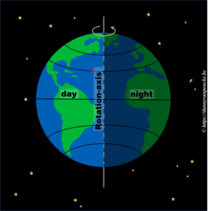
Our place on earth

To answer these questions, we need a good model of the world around us. And as is usual in science, the more accurate the model, the more detailed the answer.

Let us start very simple. We know the earth is spherical, and revolves around it’s axis in 24h. The side receiving sunlight we call day, while the shaded side is called night. If we assume the earth rotates at a constant speed, then any point on its surface will move around the earths rotational axis at a constant angular speed. This point will spend 50% of its time at the light side, and 50% at the dark side. Here we have also silently assumed, the rotational axis of the earth is “straight up” with regard to the sun.

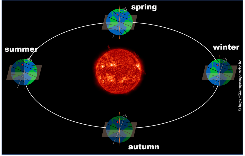
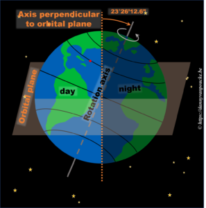
In reality, this is actually not the case. The earths rotational axis is tilted by about 23° from an axis perpendicular to the orbital plane. If we now consider a fixed point on the earths surface, we’ll note that such a point at the equator still spends 50% of its time in the light, and 50% of its time in the dark. In contrast, a point on the northern hemisphere will spend less than 50% of its time on the daylight side, while a point on the southern hemisphere spends more than 50% of its time on the daylight side. You also note that the latitude plays an important role. The more you go north, the smaller the daylight section of the latitude circle becomes, until it vanishes at the polar circle. On the other hand, on the southern hemisphere, if you move below the polar circle, the point spend all its time at the daylight side. So if the earths axis was fixed with regard to the sun, as shown in the picture, we would have a region on earth living an eternal night (north pole) or day (south pole). Luckily this is not the case. If we look at the evolution of the earths axis, we see that it is “fixed with regard to the fixed stars”, but makes a full circle during one orbit around the sun.* When the earth axis points away from the sun, it is winter on the northern hemisphere, while during summer it points towards the sun. In between, during the equinox, the earth axis points parallel to the sun, and day and night have exactly the same length: 12h.

So, now that we know the length of our daytime varies with the latitude and the time of the year, we can move one step further.

How does the length of a day vary, during the year?

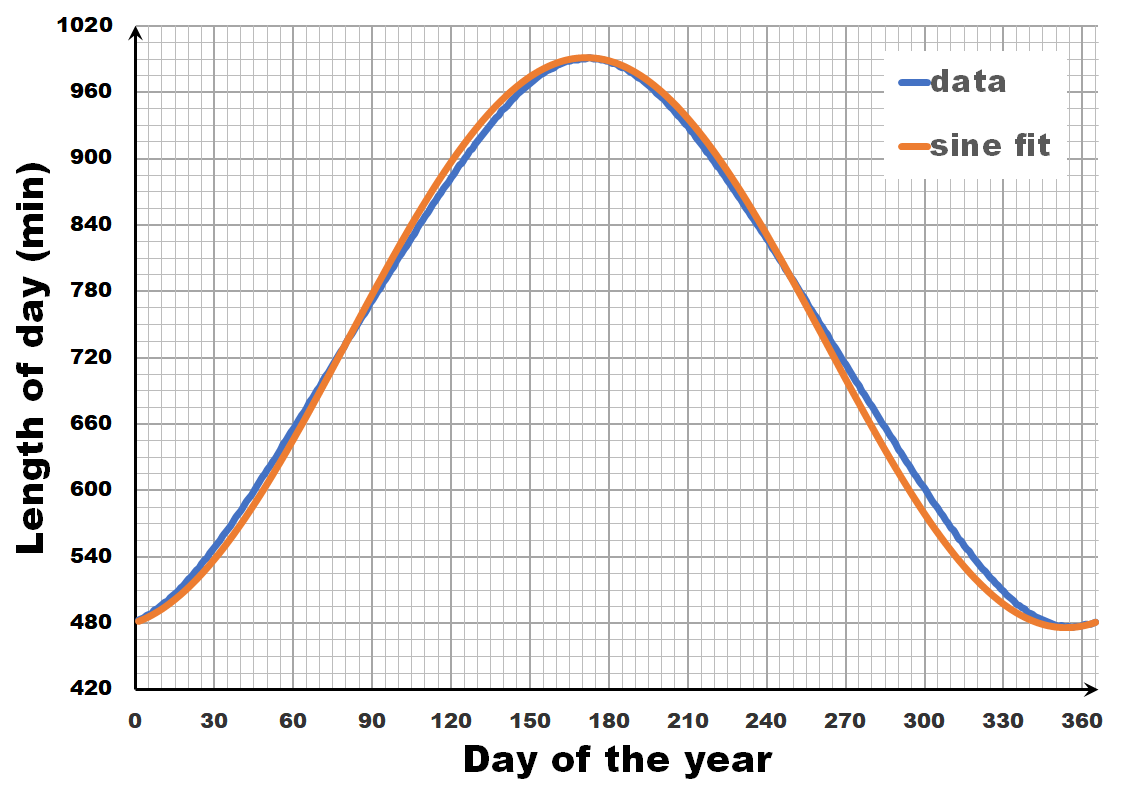
The length of the day varies over the year, with the longest and shortest days indicated by the summer and winter solstice. The periodic nature of this variation may give you the inclination to consider it as a sine wave, a sine-in-the-wild so to speak. Now let us compare a sine wave fitted to actual day-time data for Brussels. As you can see, the fit is performing quite well, but there is a clear discrepancy. So we can, and should do better than this.

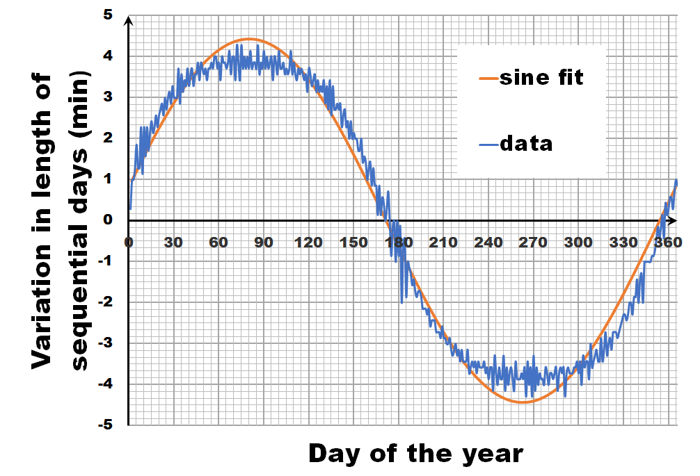
Instead of looking at the length of each day, let us have a look at the difference in length between sequential days.** If we calculate this difference for the fitted sine wave, we again get a sine wave as we are taking a finite difference version of the derivative. In contrast, the actual data shows not a sine wave, but a broadened sine wave with flat maximum and minimum. You may think this is an error, or an artifact of our averaging, but in reality, this trend even depends on the latitude, becoming more extreme the closer you get to the poles.

This additional information, provides us with the extra hint that in addition to the axial tilt of the earth axis, we also need to consider the latitude of our position. What we need to calculate is the fraction of our latitude circle (e.g. for Brussels this is 50.85°) that is illuminated by the sun, each day of the year. With some perseverance and our high school trigonometric equations, we can derive an analytic solution, which can then be calculated by, for example, excel.

Some calculations

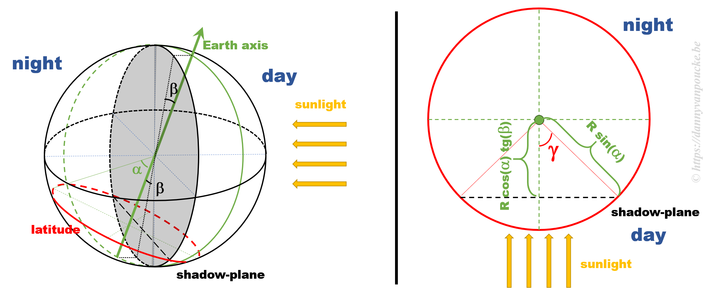
The figure above shows a 3D sketch of the situation on the left, and a 2D representation of the latitude circle on the right. α is related to the latitude, and β is the angle between the earth axis and the ‘shadow-plane’ (the plane between the day and night sides of earth). As such, β will be maximal during solstice (±23°26’12.6″) and exactly equal to zero at the equinox—when the earth axis lies entirely in the shadow-plane. This way, the length of the day is equal to the illuminated fraction of the latitude circle: 24h(360°-2γ). γ can be calculated as cos(γ)=adjacent side/hypotenuse in the right hand side part of the figure above. If we indicate the earth radius as R, then the hypotenuse is given by Rsin(α). The adjacent side, on the other hand, is found to be equal to R’sin(β), where R’=B/cos(β), and B is the perpendicular distance between the center of the earth and the plane of the latitude circle, or B=Rcos(α).

Combining all these results, we find that the number of daylight hours is:

24h*{360°-2arccos[cotg(α)tg(β)]}


How accurate is this model?

All our work is done, the actual calculation with numbers is a computer’s job, so we put excel to work. For Brussels we see that our model curve very nicely and smoothly follows the data (There is no fitting performed beyond setting the phase of the model curve to align with the data). We see that the broadening is perfectly shown, as well as the perfect estimate of the maximum and minimum variation in daytime (note that this is not a fitting parameter, in contrast to the fit with the sine wave). If you want to play with this model yourself, you can download the excel sheet here. While we are on it, I also drew some curves for different latitudes. Note that beyond the polar circles this model can not work, as we enter regions with periods of eternal day/night.


After all these calculations, be honest:

You are happy you only need to change the clock twice a year, don’t you. 🙂


* OK, in reality the earths axis isn’t really fixed, it shows a small periodic precession with a period of about 41000 years. For the sake of argument we will ignore this.

** Unfortunately, the data available for sunrises and sunsets has only an accuracy of 1 minute. By taking averages over a period of 7 years, we are able to reduce the noise from ±1 minute to a more reasonable value, allowing us to get a better picture of the general trend.

External links

Newsflash: Materials of the Future

This summer, I had the pleasure of being interviewed by Kim Verhaeghe, a journalist of the EOS magazine, on the topic of “materials of the future“. Materials which are currently being investigated in the lab and which in the near or distant future may have an enormous impact on our lives. While brushing up on my materials (since materials with length scales of importance beyond 1 nm are generally outside my world of accessibility), I discovered that to cover this field you would need at least an entire book just to list the “materials of the future”. Many materials deserve to be called materials of the future, because of their potential. Also depending on your background other materials may get your primary attention.

In the resulting article, Kim Verhaeghe succeeded in presenting a nice selection, and I am very happy I could contribute to the story. Introducing “the computational materials scientist” making use of supercomputers such as BrENIAC, but also new materials such as Metal-Organic Frameworks (MOF) and shedding some light on “old” materials such as diamond, graphene and carbon nanotubes.

Dangerous travel physics

Tossing coins into a fountain brings luck, tossing them of a building causes death and destruction?


We have probably all done it at one point when traveling: thrown a coin into a wishing well or a fountain. There are numerous wishing wells with legends describing how the deity living in the well will bring good fortune in return for this gift. The myths and legends often originate from Celtic, German or Nordic traditions.

In case of the Trevi fountain, there is the belief that if you throw a coin over your left shoulder using your right hand, you will return to Rome…someday. As this fountain and legend are iconic parts of our western movie history, many, many coins get tossed into it (more than 1 Million € worth each year, which is collected an donated to charity).

In addition to these holiday legends, there also exist more recent “coin-myths”: Death by falling penny. These myths are always linked to tall buildings, and claim that a penny dropped from the top of such a building could kill someone if they hit him.

Traveling with Newton

In both kinds of coin legends, the trajectory of the coin can be predicted quite well using Newton’s Laws. Their speed is low compared to the speed of light, and the coins are sufficiently large to keep the world of quantum mechanics hidden from sight.

The second Law of Newton states that the speed of an object changes if there is a force acting on it. Here on earth, gravity is a major player (especially for Physics exercises). In case of a coin tossed into a fountain, gravity will cause the coin to follow a roughly parabolic path before disappearing into the water. The speed at which the coin will hit the water will be comparable to the speed with which it was thrown…at least if there isn’t to much of a difference in height between the surface of the water and the hand of the one throwing the coin.

But, what if this difference is large? Such as in case of the penny being dropped from a tall building. In such a case, the initial velocity is zero, and the penny is accelerated toward the ground by gravity. Using the equations of motion for a uniform accelerated system, we can calculate easily the speed at which the coin hits the ground:

x = x0 + v0*t + ½ * g * t²

v=v0+g*t

If we drop a penny from the 3rd floor of the Eiffel Tower (x0=276.13m, x=0m, v0=0 m/s, g=-9.81m/s²) then the first equation teaches us that after 7.5 seconds, the penny will hit the ground with a final speed (second equation) of -73.6 m/s (or -265 km/h)*. With such a velocity, the penny definitely will leave an impression. More interestingly, we will get the exact same result for a pea (cooked or frozen), a bowling ball, a piano or an anvil…but also a feather. At this point, your intuition must be screaming at you that you are missing something important.

All models are wrong…but they can be very useful

The power of models in physics, originates from keeping only the most important and relevant aspects. Such approximations provide a simplified picture and allow us to understand the driving forces behind nature itself. However, in this context, models in physics are approximations of reality, and thus by definition wrong, in the sense that they do not provide an “exact” representation of reality. This is also true for Newton’s Laws, and our application above. With these simple rules, it is possible to describe the motion of the planets as well as a coin tossed into the Trevi fountain.

So what’s the difference between the coin tossed into a fountain and planetary motion on the one hand, and our assorted objects being dropped from the Eiffel Tower on the other hand?

Friction as it presents itself in aerodynamic drag!

Aerodynamic drag gives rise to a force in the direction opposite to the movement, and it is defined as:

FD= ½ *Rho*v²*CD*A

This force depends on the density Rho of the medium (hence water gives a larger drag than air), the velocity and surface area A in the direction of movement of the object, and CD the drag coefficient, which depends on the shape of the object.

If we take a look at the planets and the coin tosses, we notice that, due to the absence of air between the planets, no aerodynamic drag needs to be considered for planetary motion. In case of a coin being tossed into the Trevi fountain, there is aerodynamic drag, however, the speeds are very low as well as the distance traversed. As such the effect of aerodynamic drag will be rather small, if not negligible. In case of objects being dropped from a tall building, the aerodynamic drag will not be negligible, and it will be the factors CD and A which will make sure the anvil arrives at the ground level before the feather.

Because this force also depends on the velocity, you can no longer make direct use of the first two equations to calculate the time of impact and velocity at each point of the path. You will need a numerical approach for this (which is also the reason this is not (regularly) taught in introductory physics classes at high school). However, using excel, you can get a long way in creating a numerical solution for this problem.[Excel example]

As we know the density of air is about 1.2kg/m³, CD for a thin cylinder (think coin) is 1.17, the radius of a penny is 9.5 mm and its mass is 2.5g, then we can find the terminal velocity of the penny to be 11.1 m/s (40 km/h). The penny will land on the ground after about 25.6 seconds. This is quite a bit slower than what we found before, and also quite a bit more safe. The penny will reach its terminal velocity after having fallen about 60 m, which means that dropping a penny from taller buildings (the Atomium [102 m], the Eiffel Tower [276.13 m, 3rd floor, 324 m top], the Empire State Building [381 m] or even the Burj Khalifa [829.8 m]) will have no impact on the velocity it will have when hitting the ground: 40km/h.

This is a collision you will most probably survive, but which will definitely leave a small bruise on impact.


*The minus sign indicates the coin is falling downward.

Building bridges towards experiments.

Quantum Holy Grail: The Ground-State

Quantum mechanical calculations provide a powerful tool to investigate the world around us. Unfortunately it is also a computationally very expensive tool to use, which puts a boundary on what is possible in terms of computational materials research. For example, when investigating a solid at the quantum mechanical level, you are limited in the number of atoms that you can consider. Even with a powerful supercomputer at hand, a hundred to a thousand atoms are currently accessible for “routine” investigations. The computational cost also limits the number of configurations/combinations you can calculate.

However, in the end— and often with some blood sweat and tears—these calculations do provide you the ground-state structure and energy of your system. From this point forward you can continue characterizing its properties, life is beautiful and happy times are just beyond the horizon. At this horizon your experimental colleague awaits you. And he/she tells you:

Sorry, I don’t find that structure in my sample.

After recovering from the initial shock, you soon realize that in (materials science) experiments one seldom encounters a sample in “the ground-state”. Experiments are performed at temperatures above 0K and pressures above 0 Pa (even in vacuum :p ). Furthermore, synthesis methods often involve elevated temperatures, increased pressure, mechanical forces, chemical reactions,… which give rise to meta-stable configurations. In such an environment, your nicely deduced ground-state may be an exception to the rule. It is only one point within the phase-space of the possible.

So how can you deal with this? You somehow need to sample the phase-space available to the experiment.

Sampling Phase-Space for Ball-milling synthesis.

For a few years now, I have a very fruitful collaboration with Prof. Rounaghi. His interest goes toward the cheap fabrication of metal-nitrides. Our first collaboration focused on AlN, while later work included Ti, V and Cr-nitrides. Although this initial work had a strong focus on simple corroboration through the energies calculated at the quantum mechanical level, the collaboration also allowed me to look at my data in a different way. I wanted to “simulate” the reactions of ball-milling experiments more closely.

Due to the size-limitations of quantum mechanical calculations I played with the following idea:

  • Assume there exists a general master reaction which describes what happens during ball-milling.

X Al + Y Melamine → x1 Al + x2 Melamine + x3 AlN + …

where all the xi represent the fractions of the reaction products present.

  • With the boundary condition that the number of particles needs to be conserved, you end up with a large set of (x1,x2,x3,…) configurations which each have a certain energy. This energy is calculated using the quantum mechanical energies of each product. The configuration with the lowest energy is the ground state configuration. However, investigating the entire accessible phase-space showed that the energies of the other possible configurations are generally not that much higher.
  • What if we used the energy available due to ball-milling in the same fashion as we use kBT? And sample the phase-space using Boltzmann statistics.
  • The resulting Boltzmann distribution of the configurations available in the phase-space can then be used to calculate the mass/atomic fraction of each of the products and allow us to represent an experimental sample as a collection of small units with slightly different configurations, weighted according to their Boltzmann distribution.

This setup allowed me to see the evolution in end-products as function of the initial ratio in case of AlN, and in our current project to indicate the preferred Iron-nitride present.

Grid-sampling vs Monte-Carlo-sampling

Whereas the AlN system was relatively easy to investigate—the phase space was only 3 dimensional— the recent iron based system ended up being 4 dimensional when considering only host materials, and 10 dimensional when including defects. For a small 3-4D phase-space, it is possible to create an equally spaced grid and get converged results using a few million to a billion grid-points. For a 10D phase-space this is no longer possible. As you can no longer keep all data-points (easily) in storage during your calculation (imagine 1 Billion points, requiring you to store 11 double precision floats or about 82Gb) you need a method that does not rely on large arrays of data. For our Boltzmann statistics this gives us a bit of a pickle, as we need to have the global minimum of our phase space. A grid is too course to find it, while a simple Monte-Carlo just keeps hopping around.

Using Metropolis’s improvement of the Monte-Carlo approach was an interesting exercise, as it clearly shows the beauty and simplicity of the approach. This becomes even more awesome the moment you imagine the resources available in those days. I noted 82Gb being a lot, but I do have access to machines with those resources; its just not available on my laptop. In those days MANIAC supercomputers had less than 100 kilobyte of memory.

Although I theoretically no longer need the minimum energy configuration, having access to that information is rather useful. Therefore, I first search the phase-space for this minimum. This is rather tricky using Metropolis Monte Carlo (of course better techniques exist, but I wanted to be a bit lazy), and I found that in the limit of T→0 the algorithm will move toward the minimum. This, however, may require nearly 100 million steps of which >99.9% are rejected. As it only takes about 20 second on a modern laptop…this isn’t a big issue.

Finding a minimum using Metropolis Monte Carlo.

Finding a minimum using Metropolis Monte Carlo.

Next, a similar Metropolis Monte Carlo algorithm can be used to sample the entire phase space. Using 109 sample points was already sufficient to have a nicely converged sampling of the phase space for the problem at hand. Running the calculation for 20 different “ball-milling” energies took less than 2 hours, which is insignificant, when compared to the resources required to calculate the quantum mechanical ground state energies (several years). The figure below shows the distribution of the mass fraction of one of the reaction products as well as the distribution of the energies of the sampled configurations.

Metropolis Monte Carlo distribution of mass fraction and configuration energies for 3 sets of sample points.

Metropolis Monte Carlo distribution of mass fraction and configuration energies for 3 sets of sample points.

This clearly shows us how unique and small the quantum mechanical ground state configuration and its contribution is compared to the remainder of the phase space. So of course the ground state is not found in the experimental sample but that doesn’t mean the calculations are wrong either. Both are right, they just look at reality from a different perspective. The gap between the two can luckily be bridged, if one looks at both sides of the story. 


Science Figured out

Diamond and CPU's, now still separated, but how much longer will this remain the case? Top left: Thin film N-doped diamond on Si (courtesy of Sankaran Kamatchi). Top right: Very old Pentium 1 CPU from 1993 (100MHz), with µm architecture. Bottom left: more recent intel core CPU (3GHz) of 2006 with nm scale architecture. Bottom right: Piece of single crystal diamond. A possible alternative for silicon, with 20x higher thermal conductivity, and 7x higher mobility of charge carriers.

Diamond and CPU’s, now still separated, but how much longer will this remain the case?
Top left: Thin film N-doped diamond on Si (courtesy of Sankaran Kamatchi). Top right: Very old Pentium 1 CPU from 1993 (100MHz), with µm architecture. Bottom left: more recent intel core CPU (3GHz) of 2006 with nm scale architecture. Bottom right: Piece of single crystal diamond. A possible alternative for silicon, with 20x higher thermal conductivity, and 7x higher mobility of charge carriers.

Can you pitch your research in 3 minutes, this is the concept behind “wetenschap uitgedokterd/science figured out“. A challenge I accepted after the fun I had at the science-battle. If I can explain my work to a public of 6 to 12 year-olds, explaining it to adults should be possible as well. However, 3 minutes is very short (although some may consider this long in the current bitesize world), especially if you have to explain something far from day-to-day life and can not assume any scientific background.

Where to start? Capture the imagination: “Imagine a world where you are a god.

Link back to the real world. “All modern-day high-tech toys are more and more influenced by the atomic scale details.” Over the last decade, I have seen the nano-scale progress slowly but steadily into the realm of real-life materials research. This almost invisible trend will have a huge impact on materials science in the coming decade, because more and more we will see empirical laws breaking down, and it will become harder and harder to fit trends of materials using a classical mindset, something which has worked marvelously for materials science during the last few centuries. Modern and future materials design (be it solar cells, batteries, CPU’s or even medicine) will have to rely on quantum mechanical intuition and hence quantum mechanical simulations. (Although there is still much denial in that regard.)

Is there a problem to be solved? Yes indeed: “We do not have quantum mechanical intuition by nature, and manipulating atoms is extremely hard in practice and for practical purposes.” Although popular science magazines every so often boast pictures of atomic scale manipulation of atoms and the quantum regime, this makes it far from easy and common inside and outside the university lab. It is amazing how hard these things tend to get (ask your local experimental materials research PhD) and the required blood, sweat and tears are generally not represented in the glory-parade of a scientific publication.

Can you solve this? Euhm…yes…at least to some extend. “Computational materials research can provide the quantum mechanical intuition we human beings lack, and gives us access to atomic scale manipulation of a material.” Although computational materials science is seen by experimentalists as theory, and by theoreticians as experiments, it is neither and both. Computational materials science combines the rigor and control of theory, with access to real-life systems of experiments. It, unfortunately also suffers the limitations of both: as the system is still idealized (but to much lesser extend than in theoretical work) and control is not absolute (you have to follow where the algorithms take you, just as an experimentalist has to follow where the reaction takes him/her). But, if these strengths and weaknesses are balanced wisely (requires quite a few years of experience) an expert will gain fundamental insights in experiments.

Animation representing the buildup of a diamond surface in computational work.

Animation representing the buildup of a diamond surface in computational work.

As a computational materials scientist, you build a real-life system, atom by atom, such that you know exactly where everything is located, and then calculate its properties based on the rules of quantum mechanics, for example. In this sense you have absolute control as in theory. This comes at a cost (conservation of misery 🙂 ); where nature itself makes sure the structure is the “correct one” in experiments, you have to find it yourself in computational work. So you generally end up calculating many possible structural combinations of your atoms to first find out which is the one most probable to represent nature.

So what am I actually doing?I am using atomic scale quantum mechanical computations to investigate the materials my experimental colleagues are studying, going from oxides to defects in diamond.” I know this is vague, but unfortunately, the actual work is technical. Much effort goes into getting the calculations to run in the direction you want them to proceed (This is the experimental side of computational materials science.). The actual goal varies from project to project. Sometimes, we want to find out which material is most stable, and which material is most likely to diffuse into the other, while at other times we want to understand the electronic structure, to test if a defect is really luminescent, this to trace the source of the experimentally observed luminescence. Or if you want to make it more complex, even find out which elements would make diamond grow faster.

Starting from this, I succeeded in creating a 3-minute pitch of my research for Science Figured out. The pitch can be seen here (in Dutch, with English subtitles that can be switched on through the cogwheel in the bottom right corner).

Some external links:


VSC User Day 2018

Today, I am attending the 4th VSC User Day at the “Paleis de Academiën” in Brussels. Flemish researchers for whom the lifeblood of their research flows through the chips of a supercomputer are gathered here to discuss their experiences and present their research.

Some History

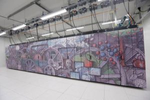
About 10 years ago, at the end of 2007 and beginning of 2008, the 5 Flemish universities founded the Flemish Supercomputer Center (VSC). A virtual organisation with one central goal:  Combine their strengths and know-how with regard to High Performance Compute (HPC) centers to make sure they were competitive with comparable HPC centers elsewhere.

By installing a super-fast network between the various university compute centers, each Flemish researcher has nowadays access to state-of-the-art computer infrastructure, independent of his or her physical location. A researcher at the University of Hasselt, like myself, can easily run calculations on the supercomputers installed at the university of Ghent or Leuven. In October 2012 the existing university supercomputers, so-called Tier-2 supercomputers, are joined by the first Flemish Tier-1 supercomputer, which was housed at the brand new data-centre of Ghent University. This machine is significantly larger than the existing Tier-2 machines, and allows Belgium to become the 25th member of the PRACE network, a European network which provides computational researchers access to the best and largest computer facilities in Europe. The fast development of computational research in Flanders and the explosive growth in the number of computational researchers, combined with the first shared Flemish supercomputer (in contrast to the university TIER-2 supercomputers, which some still consider private property rather than part of VSC) show the impact of the virtual organisation that is the VSC. As a result, on January 16th 2014, the first VSC User Day is organised, bringing together HPC users from all 5 universities  and industry. Here the users share their experiences and discuss possible improvements and changes. Since then, the first Tier-1 supercomputer has been decommissioned and replaced by a brand new Tier-1 machine, this time located at the KU Leuven. Furthermore, the Flemish government has put 30M€ aside for super-computing in Flanders, making sure that also in the future Flemish computational research stays competitive. The future of computational research in Flanders looks bright.

Today is User Day 2018

During the 4th VSC User Day, researchers of all 5 Flemish universities will be presenting the work they are performing on the supercomputers of the VSC network. The range of topics is very broad: from first principles materials modelling to chip design, climate modelling and space weather. In addition there will also be several workshops, introducing new users to the VSC and teaching advanced users the finer details of GPU-code and code optimization and parallelization. This later aspect is hugely important during the use of supercomputers in an academic context. Much of the software used is developed or modified by the researchers themselves. And even though this software can present impressive behavior, it doe not speed up automatically if you provide it access to more CPU’s. This is a very non-trivial task the researchers has to take care of, by carefully optimizing and parallelizing his or her code.

To support the researchers in their work, the VSC came up with ingenious poster-prizes. The three best posters will share 2018 node days of calculation time (about 155 years of calculations on a normal simple computer).

Wish me luck!


Single-slide presentation of my poster @VSC User Day 2018.

Single-slide presentation of my poster @VSC User Day 2018.

Fairy tale science or a science fairy tale?

Once upon a time…

Once upon a time, a long time ago—21 days ago to be precise—there was a conference in the tranquil town of Hasselt. Every year, for 23 years in a row, researchers gathered there for three full days, to present and adore their most colorful and largest diamonds. For three full days, there was just that little bit more of a sparkle to their eyes. They divulged where new diamonds could be found, and how they could be used. Three days to could speak without any restriction, without hesitation, about the sixth element which bonds them all. Because all knew the language. They honored the magic of the NV-center and the arcane incantations leading to the highest doping. All, masters of their common mystic craft.

At the end of the third day, with sadness in their harts they said their good-byes and went back, in small groups, to their own ivory tower, far far away. With them, however, they took a small sparkle of hope and expectation, because in twelve full moons they would reconvene. Bringing with them new and grander tales and even more sparkling diamonds, than had ever been seen before.

For most outsiders, the average conference presentation is as clear as an arcane conjuration of a mythological beast. As scientist, we are often trapped by the assumption that our unique expertise is common knowledge for our public, a side-effect of our enthusiasm for our own work.

Clear vs. accurate

In a world where science is facing constant pressure due to the financing model employed—in addition to the up-rise in “fake news” and “alternative facts”— it is important for young researchers to be able to bring their story clearly and accurately.

However, clear and accurate often have the bad habit of counteracting one-another, and as such, maintaining a good balance between the two take a lot more effort than one might expect. Focus on either one aspect (accuracy or clarity) tends to be disastrous. Conference presentations and scientific publications tend to focus on accuracy, making them not clear at all for the non-initiate. Public presentations and news paper articles, on the other hand, focus mainly on clarity with fake news accidents waiting to happen. For example, one could recently read that 7% of the DNA of the astronaut Scott Kelly had changed during a space-flight, instead of a change of in gene-expression. Although both things may look similar, they are very different. The latter presents a rather natural response of the (human) body to any stress situation. The former, however, removes Scott from the human race entirely. Even the average gorilla would be closer related to you and I, than Scott Kelly, as they differ less than 5% in their DNA from our DNA. So keeping a good balance between clarity and accuracy is important, albeit not that easy. Time pressure plays an important role here.

Two extremes?

Wetenschapsbattle Trophy: Each of the contestants of the wetenschapsbattle received a specially designed and created hat from the children of the school judging the contest. Mine has diamonds and computers. 🙂

In the week following the diamond conference in Hasselt, I also participated in a sciencebattle. A contest in which researchers have to explain their research to a public of 6-to 12-year-olds in a time-span of 15 minutes. These kids are judge, jury and executioner of the contest so to speak. It’s a natural reflex to place these two events at the opposite ends of a scale. And it is certainly true for some aspects; The entire room volunteering spontaneously when asked for help is something which happens somewhat less often at a scientific conference. However, clarity and accuracy should be equally central aspects for both.

So, how do you explain your complex research story to a crowd of 6-to 12-year-olds? I discovered the answer during a masterclass by The Floor is Yours.  Actually, more or less the same way you should tell it to an audience of adults, or even your own colleagues. As a researcher you are a specialist in a very narrow field, which means that no-one will loose out when focus is shifted a bit more to clarity. The main problem you encounter here, however, is time. This is both the time required to tell your story (forget “elevator pitches”, those are good if you are a used-car salesman, they are not for science) as well as the time required to prepare your story (it took me a few weeks to build and then polish my story for the children).

Most of this time is spent answering the questions: “What am I actually doing?” and “Why am I doing this specifically?“. The quest for metaphors which are both clear and accurate takes quite some time. During this task you tend to suffer, as a scientist, from the combination of your need for accuracy and your deep background knowledge. These are the same inhibitors a scientist encounters when involved in a public discussion on his/her own field of expertise.

Of course you also do not want to be pedantic:

Q: What do you do?

A: I am a Computational Materials Researcher.

Q: Compu-what??

A: 1) Computational = using a computer

2) Materials = everything you see around you, the stuff everything is made of

3) Researcher = Me

However, as a scientist, you may want to use such imaginary discussions during your preparation. Starting from these pedantic dialogues, you trace a path along the answers which interest you most. The topics which touch your scientific personality. This way, you take a step back from your direct research, and get a more broad picture. Also, by telling about theme’s, you present your research from a more broad perspective, which is more easily accessible to your audience: “What are atoms?“, “How do you make diamond?“, “What is a computer simulation?

At the end—after much blood, sweat and tears—your story tells something about your world as a whole. Depending on your audience you can include more or less detailed aspects of your actual day-to-day research, but at its hart, it remains a story.

Because, if we like it or not, in essence we all are “Pan narrans“, storytelling apes.