Category: blog

Newsflash: Book-chapter on MOFs and Zeolites en route to bookstores near you.

It is almost a year ago that I wrote a book-chapter, together with Bartek Szyja, on MOFs and Zeolites. Coming March 2018, the book will be available through University press. It is interesting to note that in a 13 chapter book, ours was the only chapter dealing with the computational study and simulation of these materials…so there is a lot more that can be done by those who are interested and have the patience to perform these delicate and often difficult but extremely rewarding studies. From my time as a MOF researcher I have learned two important things:

  1. Any kind of interesting/extreme/silly physics you can imagine will be present in some MOFs. In this regard, the current state of the MOF/COF field is still in its infancy as most experimental work focuses on  simple applications such as catalysis and gas storage, for which other materials may be better suited. These porous materials may be theoretically interesting for direct industrial application, but the synthesis cost generally will be a bottleneck. Instead, looking toward the fundamental physics applications: Low dimensional magnetism, low dimensional conduction, spin-filters, multiferroics, electron-phonon interactions, interactions between spin and mechanical properties,…. MOFs are a true playground for the theoretician.
  2. MOFs are very hard to simulate correctly, so be wary of all (published) results that come computationally cheap and easy. Although the unit-cell of any MOF is huge, with regard to standard solid state materials, the electron interactions are also quite long range, so the first Brillouin zone needs very accurate sampling (something often neglected). Also spin-configurations can have a huge influence, especially in systems with a rather flat potential energy surface.

In the book-chapter, we discuss some basic techniques used in the computational study of MOFs, COFs, and Zeolites, which will be of interest to researchers starting in the field. We discuss molecular dynamics and Monte Carlo, as well as Density Functional Theory and all its benefits and limitations.

Open Access version of the book.

A Spectre and Meltdown victim: VASP

Over the last weekend, two serious cyber security issues were hot news: Meltdown and Spectre [more links, and links](not to be mistaken for a title of a bond-movie). As a result, also academic HPC centers went into overdrive installing patches as fast as possible. The news of the two security issues went hand-in-hand with quite a few belittling comments toward the chip-designers ignoring the fact that no-one (including those complaining now) discovered the problem for over decade. Of course there was also the usual scare-mongering (cyber-criminals will hack our devices by next Monday, because hacks using these bugs are now immediately becoming their default tools etc.) typical since the beginning of the  21st century…but now it is time to return back to reality.

One of the big users on scientific HPC installations is the VASP program(an example), aimed at the quantum mechanical simulation of materials, and a program central to my own work. Due to an serendipitous coincidence of a annoyingly hard to converge job I had the opportunity to see the impact of the Meltdown and Spectre patches on the performance of VASP: 16% performance loss (within the range of the expected 10-50% performance loss for high performance applications [1][2][3]).

The case:

  • large HSE06 calculation of a 71 atom defective ZnO supercell.
  • 14 irreducible k-points (no reduction of the Hartree-Fock k-points)
  • 14 nodes of 24 cores, with KPAR=14, and NPAR=1 (I know NPAR=24 is the recommended option)

The calculation took several runs of about 10 electronic steps (of each about 5-6 h wall-time, about 2.54 years of CPU-time per run) . The relative average time is shown below (error-bars are the standard deviation of the times within a single run). As the final step takes about 50% longer it is treated separately. As you can see, the variation in time between different electronic steps is rather small (even running on a different cluster only changes the time by a few %). The impact of the Meltdown/Spectre patch gives a significant impact.

Impact of Meltdown/Spectre patch on VASP performance

Impact of Meltdown/Spectre patch on VASP performance for a 336 core MPI job.


The HPC team is currently looking into possible workarounds that could (partially) alleviate the problem. VASP itself is rather little I/O intensive, and a first check by the HPC team points toward MPI (the parallelisation framework required for multi-node jobs) being ‘a’ if not ‘the’ culprit. This means that also an impact on other multi-node programs is to be expected. On the bright side, finding a workaround for MPI would be beneficial for all of them as well.

So far, tests I performed with the HPC team not shown any improvements (recompiling VASP didn’t help, nor an MPI related fix). Let’s keep our fingers crossed, and hope the future brings insight and a solution.


Review of 2017

Happy New Year

2017 has come and gone. 2018 eagerly awaits getting acquainted. But first we look back one last time, trying to turn this into a old tradition. What have I done during the last year of some academic merit.

Publications: +4

Completed refereeing tasks: +8

  • The Journal of Physical Chemistry (2x)
  • Journal of Physics: Condensed Matter (3x)
  • Diamond and Related Materials (3x)

Conferences & workshops: +5 (Attended) 

  • Int. Conference on Diamond and Carbon Materials (DCM) 2017, Gothenburg, Sweden, September 3rd-7th, 2017 [oral presentation]
  • Summerschool: “Upscaling techniques for mathematical models involving multiple scales”, Hasselt, Belgium, June 26th-29th, 2017 [poster presentation]
  • VSC-user day, Brussels, Belgium, June 2nd, 2017 [poster presentation]
  • E-MRS 2017 Spring Meeting, Strasbourg, France, May 22nd-26th, 2017 [1 oral + 2 poster presentations]
  • SBDD XXII, Hasselt University, Belgium, March 8th-10th, 2017 [poster presentation]

PhD-students: +1

  • Mohammadreza Hosseini (okt.-… ,Phd student physical chemistry, Tarbiat Modares University, Teheran, Iran)

Bachelor-students: +2

Current size of HIVE:

  • 48.5K lines of program (code: 70 %)
  • ~70 files
  • 45 (command line) options

Hive-STM program:

And now, upward and onward, a new year, a fresh start.

Slow science: the case of Pt induced nanowires on Ge(001)

Free-standing Pt-induced nanowire on Ge(001).

Simulated STM image of the Pt-induced nanowires on the Ge(001) surface. Green discs indicate the atomic positions of the bulk-Ge atoms; red: Pt atoms embedded in the top surface layers; yellow: Ge atoms forming the nanowire observed by STM.

Ten years ago, I was happily modeling Pt nanowires on Ge(001) during my first Ph.D. at the university of Twente. As a member of the Computational Materials Science group, I also was lucky to have good and open contact with the experimental research group of Prof. Zandvliet, whom was growing these nanowires. In this environment, I learned there is a big difference between what is easy in experiment and what is easy in computational research. It also taught me to find a common ground which is “easy” for both (Scanning tunneling microscopy (STM) images in this specific case).

During this 4-year project, I quickly came to the conclusion that the nanowires could not be formed by Pt atoms, but that it needed to be Ge atoms instead. Although the simulated STM images were  very convincing, it was really hard to overcome the experimental intuition…and experiments which seemed to contradict this picture (doi: 10.1016/j.susc.2006.07.055 ). As a result, I spend a lot of time learning about the practical aspects of the experiments (an STM tip is a complicated thing) and trying to extract every possible piece of information published and unpublished. Especially the latter provided important support. The “ugly”(=not good for publishing) experimental pictures tended to be real treasures from my computational point of view. Of course, much time was spent on tweaking the computational model to get a perfect match with experiments (e.g. the 4×1 periodicity), and trying to reproduce experiments seemingly supporting the “Ge-nanowire” model (e.g. simulation of CO adsorption and identification of the path along the wire the molecule follows.).

In contrast to my optimism at the end of my first year (I believed all modeling could be finished before my second year ended), the modeling work ended up being a very complex exercise, taking 4 years of research. Now I am happy that I was wrong, as the final result ended up being very robust and became “The model for Pt induced nanowires on Ge(001)“.

Upon doing a review article on this field five years after my Ph.D. I was amazed (and happy) to see my model still stood. Even more, there had been complex experimental studies (doi: 10.1103/PhysRevB.85.245438) which even seemed to support the model I proposed. However, these experiments were stil making an indirect comparison. A direct comparison supporting the Ge nature of the nanowires was still missing…until recently.

In a recent paper in Phys. Rev. B (doi: 10.1103/PhysRevB.96.155415) a Japanese-Turkish collaboration succeeded in identifying the nanowire atoms as Ge atoms. They did this using an Atomic Force Microscope (AFM) and a sample of Pt induced nanowires, in which some of the nanowire atoms were replaced by Sn atoms. The experiment rather simple in idea (execution however requires rather advanced skills): compare the forces experienced by the AFM when measuring the Sn atom, the chain atoms and the surface atoms. The Sn atoms are easily recognized, while the surface is known to consist of Ge atoms. If the relative force of the chain atom is the same as that of the surface atoms, then the chain consists of Ge atoms, while if the force is different, the chain consists of Pt atoms.

*small drum-roll*

And they found the result to be the same.

Yes, after nearly 10 years since my first publication on the subject, there finally is experimental proof that the Pt nanowires on Ge(001) consist of Ge atoms. Seeing this paper made me one happy computational scientist. For me it shows the power of computational research, and provides an argument why one should not be shy to push calculations to their limit. The computational cost may be high, but at least one is performing relevant work. And of course, never forget, the most seemingly easy looking experiments are  usually not easy at all, so as a computational materials scientist you should not take them for granted, but let those experimentalists know how much you appreciate their work and effort.

Audioslides tryout.

One of the new features provided by Elsevier upon publication is the creation of audioslides. This is a kind of short presentation of the publication by one of the authors. I have been itching to try this since our publication on the neutral C-vancancy was published. The interface is quite intuitive, although the adobe flash tend to have a hard time finding the microphone. However, once it succeeds, things go quite smoothly. The resolution of the slides is a bit low, which is unfortunate (but this is only for the small-scale version, the large-scale version is quite nice as you can see in the link below). Maybe I’ll make a high resolution version video and put it on Youtube, later.

The result is available here (since the embedding doesn’t play nicely with WP).

And a video version can be found here.
 

Exa-scale computing future in Europe?

As a computational materials scientist with a main research interest in the ab initio simulation of materials, computational resources are the life-blood of my research. Over the last decade, I have seen my resource usage grow from less than 100.000 CPU hours per year to several million CPU-hours per year. To satisfy this need for computational resources I have to make use of HPC facilities, like the TIER-2 machines available at the Flemish universities and the Flemish TIER-1 supercomputer, currently hosted at KU Leuven. At the international level, computational scientists have access to so called TIER-0 machines, something I no doubt will make use of in the future. Before I continue, let me first explain a little what this TIER-X business actually means.

The TIER-X notation is used to give an indication of the size of the computer/supercomputer indicated. There are 4 sizes:

  •  TIER-3: This is your personal computer(laptop/desktop) or even a small local cluster of a research group. It can contain from one (desktop) up to a few hundred CPU’s (local cluster). Within materials research, this is sufficient for quite a few tasks: post-processing of data, simple force-field based calculations, or even small quantum chemical or solid state calculations. A large fraction of the work during my first Ph.D. was performed on the local cluster of the CMS.
  • TIER-2: This is a supercomputer hosted by an institute or university. It generally contains over 1000 CPUs and has a peak performance of >10 TFLOPS (1012 Floating Point Operations Per Second, compare this to 1-50×10FLOPS or 1-25 GFLOPS of an average personal computer). The TIER-2 facilities of the VUB and UAntwerp both have a peak performance of about 75TFLOPS , while the machines at Ghent University and the KU Leuven/Uhasselt facilities both have a peak performance of about 230 TFLOPS. Using these machines I was able to perform the calculations necessary for my study of dopant elements in cerates (and obtain my second Ph.D.).
  • TIER-1: Moving up one more step, there are the national/regional supercomputers. These generally contain over 10.000 CPUs and have a peak performance of over 100 TFLOPS. In Flanders the Flemish Supercomputer Center (VSC) manages the TIER-1 machine (which is being funded by the 5 Flemish universities). The first TIER-1 machine was hosted at Ghent University, while the second and current one is hosted at KU Leuven, an has a peak performance of 623 TFLOPS (more than all TIER-2 machines combined), and cost about 5.5 Million € (one of the reasons it is a regional machine). Over the last 5 years, I was granted over 10 Million hours of CPU time, sufficient for my study of Metal-Organic Frameworks and defects in diamond.
  • TIER-0: This are international level supercomputers. These machines contain over 100.000 CPUs, and have a peak performance in excess of 1 PFLOP (1 PetaFLOP = 1000 TFLOPS). In Europe the TIER-0 facilities are available to researchers via the PRACE network (access to 7 TIER-0 machines, accumulated 43.49 PFLOPS).

This is roughly the status of what is available today for Flemish scientists at various levels. With the constantly growing demand for more processing power, the European union, in name of EuroHPC, has decided in march of this year, that Europe will host two Exa-scale computers. These machines will have a peak performance of at least 1 EFLOPS, or 1000 PFLOPS. These machines are expected to be build by 2024-2025. In June, Belgium signed up to EuroHPC as the eighth country participating, in addition, to the initial 7 countries (Germany, France, Spain, Portugal, Italy, Luxemburg and The Netherlands).

This is very good news for all involved in computational research in Flanders. There is the plan to build these machines, there is a deadline, …there just isn’t an idea of what these machines should look like (except: they will be big, massively power consuming and have a target peak performance). To get an idea what users expect of such a machine, Tier-1 and HPC users have been asked to put forward requests/suggestions of what they want.

From my user personal experience, and extrapolating from my own usage I see myself easily using 20 million hours of CPU time each year by the time these Exa-scale machines are build. Leading a computational group would multiply this value. And then we are talking about simple production purpose calculations for “standard” problems.

The claim that an Exa-scale scale machine runs 1000x faster than a peta-scale machine, is not entirely justified, at least not for the software I am generally encountering. As software seldom scales linearly, the speed-gain from Exa-scale machinery mainly comes from the ability to perform many more calculations in parallel. (There are some exceptions which will gain within the single job area, but this type of jobs is limited.) Within my own field, quantum mechanical calculation of the electronic structure of periodic atomic systems, the all required resources tend to grow with growth of the problem size. As such, a larger system (=more atoms) requires more CPU-time, but also more memory. This means that compute nodes with many cores are welcome and desired, but these cores need the associated memory. Doubling the cores would require the memory on a node to be doubled as well. Communication between the nodes should be fast as well, as this will be the main limiting factor on the scaling performance. If all this is implemented well, then the time to solution of a project (not a single calculation) will improve significantly with access to Exa-scale resources. The factor will not be 100x from a Pflops system, but could be much better than 10x. This factor 10 also takes into account that projects will have access to much more demanding calculations as a default (Hybrid functional structure optimization instead of simple density functional theory structure optimization, which is ~1000x cheaper for plane wave methods but is less accurate).

At this scale, parallelism is very important, and implementing this into a program is far from a trivial task. As most physicists/mathematicians/chemists/engineers may have the skills for writing scientifically sound software, we are not computer-scientists and our available time and skills are limited in this regard. For this reason, it will become more important for the HPC-facility to provide parallelization of software as a service. I.e. have a group of highly skilled computer scientists available to assist or even perform this task.

Next to having the best implementation of software available, it should also be possible to get access to these machines. This should not be limited to a happy few through a peer review process which just wastes human research potential. Instead access to these should be a mix of guaranteed access and peer review.

  • Guaranteed access: For standard production projects (5-25 million CPU hours/year) university researchers should have a guaranteed access model. This would allow them to perform state of the are research without too much overhead. To prevent access to people without the proven necessary need/skills it could be implemented that a user-database is created and appended upon each application. Upon first application, a local HPC-team (country/region/university Tier-1 infrastructure) would have to provide a recommendation with regard to the user, including a statement of the applicant’s resource usage at that facility. Getting resources in a guaranteed access project would also require a limited project proposal (max 2 pages, including user credentials, requested resources, and small description of the project)
  • Peer review access: This would be for special projects, in which the researcher requires a huge chunk of resources to perform highly specialized calculations or large High-throughput exercises (order of 250-1000 million CPU hours, e.g. Nature Communications 8, 15959 (2017)). In this case a full project with serious peer review (including rebuttal stage, or the possibility to resubmit after considering the indicated problems). The goal of this peer review system should not be to limit the number of accepted projects, but to make sure the accepted projects run successfully.
  • Pay per use: This should be the option for industrial/commercial users.

What could an HPC user as myself do to contribute to the success of EuroHPC? This is rather simple, run the machine as a pilot user (I have experience on most of the TIER-2 clusters of Ghent University and both Flemish Tier-1 machines. I successfully crashed the programs I am using by pushing them beyond their limits during pilot testing, and ran into rather unfortunate issues. 🙂 That is the job of a pilot user, use the machine/software in unexpected ways, such that this can be resolved/fixed by the time the bulk of the users get access.) and perform peer review of the lager specialized projects.

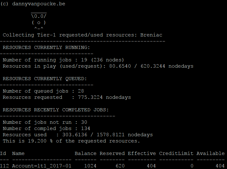
Now the only thing left to do is wait. Wait for the Exa-scale supercomputers to be build…7 years to go…about 92 node-days on Breniac…a starting grant…one long weekend of calculations.

Appendix

For simplicity I use the term CPU to indicate a single compute core, even though technically, nowadays a single CPU will contain multiple cores (desktop/laptop: 2-8 cores, HPC-compute node: 2-20 cores / CPU (or more) ). This to make comparison a bit more easy.

Furthermore, modern computer systems start more and more to rely on GPU performance as well, which is also a possible road toward Exa-scale computing.

Orders of magnitude:

  • G = Giga = 109
  • T = Tera = 1012
  • P = Peta = 1015
  • E = Exa = 1018

Just married

Today is a joyful day, as I am getting married to my lovely girlfriend, my partner in crime, the mother of our son, the stars of my night-sky: my wife.

In February, we silently snuck out and got married (just the two of us and our son). We even had a small honeymoon/pilgrimage to Enschede, the place where it all began. We visited the town and the university campus, reliving old memories of those first days.

Today, we have the ring-ceremony and wedding party to share our happiness  with our family and friends. As we are having the celebration at a local castle, Sylvia also designed a special coat of arms for our little family:


Calculemus et Sapiamus

Resource management on HPC infrastructures.

Computational as a third pillar of science (next to experimental and theoretical) is steadily developing in many fields of science. Even some fields you would less expect it, such as sociology or psychology. In other fields such as physics, chemistry or biology it is much more widespread, with people pushing the boundaries of what is possible. Larger facilities provide access to larger problems to tackle. If a computational physicist is asked if larger infrastructures would not become too big, he’ll just shrug and reply: “Don’t worry, we will easily fill it up, even a machine 1000x larger than that.” An example is given by a pair of physicists who recently published their atomic scale study of the HIV-1 virus. Their simulation of a model containing more than 64 million atoms used force fields, making the simulation orders of magnitude cheaper than quantum mechanical calculations. Despite this enormous speedup, their simulation of 1.2 µs out of the life of an HIV-1 virus (actually it was only the outer skin of the virus, the inside was left empty) still took about 150 days on 3880 nodes of 16 cores on the Titan super computer of Oak Ridge National Laboratory (think about 25 512 years on your own computer).

In Flanders, scientist can make use of the TIER-1 facilities provided by the Flemish Super Computer (VSC). The first Tier-1 machine was installed and hosted at Ghent University. At the end of it’s life cycle the new Tier-1 machine (Breniac) was installed and is hosted at KULeuven. Although our Tier-1 supercomputer is rather modest compared to the Oak Ridge supercomputer (The HIV-1 calculation I mentioned earlier would require 1.5 years of full time calculations on the entire machine!) it allows Flemish scientists (including myself) to do things which are not possible on personal desktops or local clusters. I have been lucky, as all my applications for calculation time were successful (granting me between 1.5 and 2.5 million hours of CPU time every year). With the installment of the new supercomputer accounting of the requested resources has become fully integrated and automated. Several commands are available which provide accounting information, of which mam-balance is the most important one, as it tells how much credits are still available. However, if you are running many calculations you may want to know how many resources you are actually asking and using in real-time. For this reason, I wrote a small bash-script that collects the number of requested and used resources for running jobs:

Output of the Bash Script.

Currently, the last part, on the completed jobs, only provides data based on the most recent jobs. Apparently the full qstat information of older jobs is erased. However, it still provides an educated guess of what you will be using for the still queued jobs.


Functional Molecular Modelling: simulating particles in excel

This semester I had several teaching assignments. I was a TA for the course biophysics for the first bachelor biomedical sciences, supervised two 3rd bachelor students physics during their first steps in the realm of computational materials science, and finally, I was responsible for half the course Functional Molecular Modelling for the first Masters Biomedical students (Bioelectronics and Nanotechnology). In this course, I introduce the the students into the basic concepts of classical molecular modelling (quantum modelling is covered by Prof. Wilfried Langenaeker). It starts with a reiteration of some basic concepts from statistics and moves on to cover the canonical ensemble. Things get more interesting with the introduction into Monte-Carlo(MC) and Molecular Dynamics(MD), where I hope to teach the students the basics needed to perform their own MC and MD simulations. This also touches the heart of what this course should cover. If I hear a title like Functional Molecular Modelling, my thoughts move directly to practical applications, developing and implementing models, and performing simulations. This becomes a bit difficult as none of the students have any programming experience or skills.

Luckily there is excel. As the basic algorithms for MC and MD are actually quite simple, this office package can be (ab)used to allow the students to perform very simple simulations. This even without the use of macro’s or any advanced features. Because Excel can also plot the data present in the cells, you immediately see how properties of the simulated system vary during the simulation, and you get direct update of all graphs every time a simulation is run.

It seems I am not the only one who is using excel for MD simulations. In 1995, Fraser and Woodcock even published a paper detailing the use of excel for performing MD simulations on a system of 100 particles. Their MD is a bit more advanced than the setup I used as it made heavy use of macro’s and needed some features to speed things up as much as possible. With the x486 66MHz computers available at that time, the simulations took of the order of hours. Which was impressive, as they served as an example of how computational speed had improved over the years, and compared to the months of supercomputer resources one of the authors had needed 25 years earlier to perform the same thing for his PhD. Nowadays the same excel simulation should only take minutes, while an actual program in Fortran or C may even execute the same thing in a matter of seconds or less.

For the classes and exercises, I made use of a simple 3-atom toy-model with Lennard-Jones interactions. The resulting simulations remain clear allowing their use for educational purposes. In case of  MC simulations, a nice added bonus is the fact that excel updates all its fields automatically when a cell is modified. As a result, all random numbers are regenerated and a new simulation can be performed by saving the excel-sheet or just modifying a not-used cell.

Monte Carlo in excel. A system of three particles on a line, with one particle fixed at 0. All particles interact through a Lennard-Jones potential. The Monte Carlo simulation shows how the particles move toward their equilibrium position.

Monte Carlo in excel. A system of three particles on a line, with one particle fixed at 0. All particles interact through a Lennard-Jones potential. The Monte Carlo simulation shows how the particles move toward their equilibrium position.

The simplicity of Newton’s equations of motion make it possible to perform simple MD simulations, and already for a three particle system, you can see how unstable the algorithm is. Implementation of the leap-frog algorithm isn’t much more complex and shows incredible the stability of this algorithm. In the plot of the total energy you can even see how the algorithm fights back to retain stability (the spikes may seem large, but the same setup with a straight forward implementation of Newton’s equation of motion quickly moves to energies of the order of 100).

Molecular dynamics in excel. A system of three particles on a line, with one particle fixed at 0. All particles interact through a Lennard-Jones potential. The Molecular dynamics simulation shows how the particles move as time evolves. Their positions are updated using the leap-frog algorithm. The extreme hard nature of the Lennard-Jones potential gives rise to the sharp spikes in the total energy. It is this last aspect which causes the straight forward implementation of Newton's equations of motion to fail.

Molecular dynamics in excel. A system of three particles on a line, with one particle fixed at 0. All particles interact through a Lennard-Jones potential. The Molecular dynamics simulation shows how the particles move as time evolves. Their positions are updated using the leap-frog algorithm. The extreme hard nature of the Lennard-Jones potential gives rise to the sharp spikes in the total energy. It is this last aspect which causes the straight forward implementation of Newton’s equations of motion to fail.


Bachelor Projects Completed: 2 new computational materials scientists initialised

The black arts of computational materials science.

Black arts of computational materials science.

Just over half a year ago, I mentioned that I presented two computational materials science related projects for the third bachelor physics students at the UHasselt. Both projects ended up being chosen by a bachelor student, so I had the pleasure of guiding two eager young minds in their first steps into the world of computational materials science. They worked very hard, cursed their machine or code (as any good computational scientist should do once in a while, just to make sure that he/she is still at the forefront of science) and survived. They actually did quite a bit more than “just surviving”, they grew as scientists and they grew in self-confidence…given time I believe they may even thrive within this field of research.

One week ago, they presented their results in a final presentation for their classmates and supervisors. The self-confidence of Giel, and the clarity of his story was impressive. Giel has a knack for storytelling in (a true Pan Narrans as Terry Pratchett would praise him). His report included an introduction to various topics of solid state physics and computational materials science in which you never notice how complicated the topic actually is. He just takes you along for the ride, and the story unfolds in a very natural fashion. This shows how well he understands what he is writing about.

This, in no way means his project was simple or easy. Quite soon, at the start of his project Giel actually ran into a previously unknown VASP bug. He had to play with spin-configurations of defects and of course bumped into a hand full of rookie mistakes which he only made once *thumbs-up*. (I could have warned him for them, but I believe people learn more if they bump their heads themselves. This project provided the perfect opportunity to do so in a safe environment. 😎 )  His end report was impressive and his results on the Ge-defect in diamond are of very good quality.

The second project was brought to a successful completion by Asja. This very eager student actually had to learn how to program in fortran before he could even start. He had to implement code to calculate partial phonon densities with the existing HIVE code. Along the way he also discovered some minor bugs (Thank you very much 🙂  ) and crashed into a rather unexpected hard one near the end of the project. For some time, things looked very bleak indeed: the partial density of equivalent atoms was different, and the sum of all partial densities did not sum to the total density. As a result there grew some doubts if it would be possible to even fulfill the goal of the project. Luckily, Asja never gave up and stayed positive, and after half a day of debugging on my part the culprit was found (in my part of the code as well). Fixing this he quickly started torturing his own laptop calculating partial phonon densities of state for Metal-organic frameworks and later-on also the Ge-defect in diamond, with data provided by Giel. Also these results are very promising and will require some further digging, but they will definitely be very interesting.

For me, it has been an interesting experience, and I count myself lucky with these two brave and very committed students. I wish them all the best of luck for the future, and maybe we meet again.