Tag: Materials Science

Materiomics Chronicles: week 1

The first week of the academic year at UHasselt has come to an end, while colleagues at UGent and KULeuven are still preparing for the start of their academic year next week. Good luck to all of you.

This week started full throttle for me, with classes for each of my six courses. After introductions in classes with new students (for me) in the second bachelor chemistry and first master materiomics, and a general overview in the different courses, we quickly dove into the subject at hand.

The second bachelor students got a soft introduction into (some of) the historical events leading up to the birth of quantum mechanics such as the black body radiation, the atomic model and the nature of light. They encountered the duck-rabbit of particle-wave duality and awakened their basic math skills with the standing wave problem. For the third bachelor students, the course on quantum and computational chemistry started with a quick recap of the course introduction to quantum mechanics, making sure they are all again up to speed with concepts like braket-notation and commutator relations.

For the master materiomics it was also a busy week. We kicked of the 1st Ma course “Fundamentals of modeling“, which starts of calm and easy with a general picture of the role of computational research as third research paradigm. We discussed in which fields computational research can be found (flabbergasting students with an example in Theology: a collaboration between Sylvia Wenmackers & Helen De Cruz),  approximation vs idealization, examples of materials research at different scales, etc. As a homework assignment the students were introduced into the world of algorithms through the lecture of Hannah Fry (Should computers run the world). For the  2nd Ma, the courses on DFT and AI both started. The lecture of the former focused on the nuclear wave function and how we (don’t) deal with it in DFT, but still succeed in optimizing structures. During the lecture on AI we dove into the topics of regularization and learning curves, and extended on different types of ensemble models.

At the end of week 1, this brings me to a total of 12h of lectures. Upwards and onward to week 2.

Practical Machine-Learning for the Materials Scientist

Scilight graphic

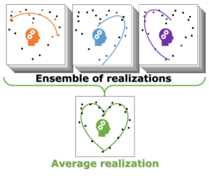
Individual model realizations may not perform that well, but the average model realization always performs very well.

Machine-Learning  is up and trending. You can’t open a paper, magazine or website without someone trying to convince you their new AI-improved app/service will radically change your life. It will make the production of your company more efficient and cheaper, make costumers flock to your shop and possibly cure cancer on the side. Also in science, a lot of impressive claims are being made. General promises entail that it makes the research of interest faster, better, more efficient,… There is, however, a bit of fine print which is never explicitly mentioned: you need a LOT of data. This data is used to teach your Machine-Learning algorithm whatever it is intended to learn.

In some cases, you can get lucky, and this data is already available while in other, you still need to create it yourself. In case of computational materials science this often means performing millions upon millions of calculations to create a data set on which to train the Machine-Learning algorithm.[1] The resulting Machine-Learning model may be a thousand times faster in direct comparison, but only if you ignore the compute-time deficit you start from.

In materials science, this is not only a problem for those performing first principles modeling, but also for experimental researchers. When designing a new material, you generally do not have the resources to generate thousands or millions of samples while varying the parameters involved. Quite often you are happy if you can create even a few dozen samples. So, can this research still benefit from Machine-Learning if only very small data sets are available?

In my recent work on materials design using Machine-Learning combined with small data sets, I discuss the limitations of small data sets in the context of Machine-Learning and present a natural approach for obtaining the best possible model.[2] [3]

The Good, the Bad and the Average.

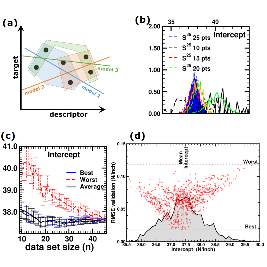
(a) Simplified representation of modeling small data sets. (b) Data set size dependence of the distribution of model coefficients. (c) Evolution of model-coefficients with data set size. (d) correlation between model coefficient value and model quality.

In Machine-Learning a data set is generally split in two parts. One part to train the model, and a second part to test the quality of the model. One of the underlying assumptions to this approach is that each subset of the data set provides an accurate representation of the “true” data/model. As a result, taking a different subset to train your data should give rise to “the same model” (ignoring small numerical fluctuations). Although this is generally true for large (and huge) data sets, for  small data sets this is seldomly the case (cf. figure (a) on the side). There, the individual data points considered will have a significant impact on the final model, and different subsets give rise to very different models. Luckily the coefficients of these models still present a peaked distribution. (cf. figure (b)).

On the down side, however, if one isn’t careful in preprocessing the data set correctly, these distributions will not converge upon increasing the data set size, giving rise to erratic model behaviour.[2]

Not only the model coefficients give rise to a distribution, the same is true for the model quality. Using the same data set, but making a different split between training and test data can give rise to large differences in  quality for the model instances. Interestingly, the model quality presents a strong correlation with the model coefficients, with the best quality model instances being closer to the “true” model instance. This gives rise to a simple approach: just take many train-test splittings, and select the best model. There are quite some problems with such an approach, which are discussed in the manuscript [2]. The most important one being the fact that the quality measure on a very small data set is very volatile itself. Another is the question of how many such splittings should be considered? Should it be an exhaustive search, or are any 10 random splits good enough (obviously not)? These problems are alleviated by the nice observation that “the average” model shows not the average quality or the average model coefficients, but instead it presents the quality of the best model (as well as the best model coefficients). (cf. figure (c) and (d))

This behaviour is caused by the fact that the best model instances have model coefficients which are also the average of the coefficient distributions. This observation hold for simple and complex model classes making it widely applicable. Furthermore, for model classes for which it is possible to define a single average model instance, it gives access to a very efficient predictive model as it only requires to store model coefficients for a single instance, and predictions only require a single evaluation. For models where this is not the case one can still make use of an ensemble average to benefit from the superior model quality, but at a higher computational cost. 

References and footnotes

[1] For example, take “ANI-1: an extensible neural network potential with DFT accuracy at force field computational cost“, one of the most downloaded papers of the journal of Chemical Science. The data set the authors generated to train their neural network required them to optimize 58.000 molecules using DFT calculations. Furthermore, for these molecules a total of about 17.200.000 single-point energies were calculated (again at the DFT level). I leave it to the reader to estimate the amount of calculation time this requires.

[2] “Small Data Materials Design with Machine Learning: When the Average Model Knows Best“, Danny E. P. Vanpoucke, Onno S. J. van Knippenberg, Ko Hermans, Katrien V. Bernaerts, and Siamak Mehrkanoon, J. Appl. Phys. 128, 054901  (2020)

[3] “When the average model knows best“, Savannah Mandel, AIP SciLight 7 August (2020)

Universiteit Van Vlaanderen: Will we be able to design new materials using our smartphone in the future?

Yesterday, I had the pleasure of giving a lecture for the Universiteit van Vlaanderen, a science communication platform where Flemish academics are asked to answer “a question related to their research“. This question is aimed to be highly clickable and very much simplified. The lecture on the other hand is aimed at a general lay public.

I build my lecture around the topic of materials simulations at the atomic scale. This task ended up being rather challenging, as my computational research has very little direct overlap with the everyday life of the average person. I deal with supercomputers (which these days tend to be bench-marked in terms of smartphone power) and the quantum mechanical simulation of materials at the atomic scale, two other topics which may ring a bell…but only as abstract topics people may have heard of.

Therefor, I crafted a story taking people on a fast ride down the rabbit hole of my work. Starting from the almost divine power of the computational materials scientist over his theoretical sample, over the reality of nano-scale materials in our day-to-day lives, past the relative size of atoms and through the game nature of simulations and the salvation of computational research by grace of Moore’s Law…to the conclusion that in 25 years, we may be designing the next generation of CPU materials on our smartphone instead of a TIER-1 supercomputer. …did I say we went down the rabbit hole?

The television experience itself was very exhilarating for me. Although my actual lecture took only 15 minutes, the entire event took almost a full day. Starting with preparations and a trial run in the afternoon (for me and my 4 colleagues) followed by make-up (to make me look pretty on television 🙂 … or just to reduce my reflectance). In the evening we had a group diner meeting the people who would be in charge of the technical aspects and entertainment of the public. And then it was 19h30. Tensions started to grow. The public entered the studio, and the show was ready to start. Before each lecture, there was a short interview to test sound and light, and introduce us to the public. As the middle presenter, I had the comfortable position not to be the first, so I could get an idea of how things went for my colleagues, and not to be the last, which can really be destructive on your nerves.

At 21h00, I was up…

and down the rabbit hole we went. 


Full periodic table, with all elements presented with their relative size (if known)

Full periodic table, with all elements presented with their relative size (if known) created for the Universiteit van Vlaanderen lecture.


Newsflash: Materials of the Future

This summer, I had the pleasure of being interviewed by Kim Verhaeghe, a journalist of the EOS magazine, on the topic of “materials of the future“. Materials which are currently being investigated in the lab and which in the near or distant future may have an enormous impact on our lives. While brushing up on my materials (since materials with length scales of importance beyond 1 nm are generally outside my world of accessibility), I discovered that to cover this field you would need at least an entire book just to list the “materials of the future”. Many materials deserve to be called materials of the future, because of their potential. Also depending on your background other materials may get your primary attention.

In the resulting article, Kim Verhaeghe succeeded in presenting a nice selection, and I am very happy I could contribute to the story. Introducing “the computational materials scientist” making use of supercomputers such as BrENIAC, but also new materials such as Metal-Organic Frameworks (MOF) and shedding some light on “old” materials such as diamond, graphene and carbon nanotubes.

Linker Functionalization in MIL-47(V)-R Metal–Organic Frameworks: Understanding the Electronic Structure

Authors: Danny E. P. Vanpoucke
Journal: J. Phys. Chem. C 121(14), 8014-8022 (2017)
doi: 10.1021/acs.jpcc.7b01491
IF(2017): 4.484
export: bibtex
pdf: <J.Phys.Chem.C>
Graphical Abstract: Evolution of the electronic band structure of MIL-47(V) upon OH-functionalization of the BDC linker.
Graphical Abstract: Evolution of the electronic band structure of MIL-47(V) upon OH-functionalization of the BDC linker. The π-orbital of the BDC linker splits upon functionalisation, and the split-off π-band moves up into the band gap, effectively reducing the latter.

Abstract

Metal–organic frameworks (MOFs) have gained much interest due to their intrinsic tunable nature. In this work, we study how linker functionalization modifies the electronic structure of the host MOF, more specifically, the MIL-47(V)-R (R = −F, −Cl, −Br, −OH, −CH3, −CF3, and −OCH3). It is shown that the presence of a functional group leads to a splitting of the π orbital on the linker. Moreover, the upward shift of the split-off π-band correlates well with the electron-withdrawing/donating nature of the functional groups. For halide functional groups the presence of lone-pair back-donation is corroborated by calculated Hirshfeld-I charges. In the case of the ferromagnetic configuration of the host MIL-47(V+IV) material a half-metal to insulator transition is noted for the −Br, −OCH3, and −OH functional groups, while for the antiferromagnetic configuration only the hydroxy group results in an effective reduction of the band gap.

MRS seminar: Topological Insulators

Bart Sorée receives a commemorative frame of the event. Foto courtesy of Rajesh Ramaneti.

Today I have the pleasure of chairing the last symposium of the year of the MRS chapter at UHasselt. During this invited lecture, Bart Sorée (Professor at UAntwerp and KULeuven, and alumnus of my own Alma Mater) will introduce us into the topic of topological insulators.

This topic became unexpectedly a hot topic as it is part of the 2016 Nobel Prize in Physics, awarded last Saturday.

This year’s Nobel prize in physics went to: David J. Thouless (1/2), F. Duncan M. Haldane (1/4) and J. Michael Kosterlitz (1/4) who received it

“for theoretical discoveries of topological phase transitions and topological phases of matter.”

On the Nobel Prize website you can find this document which gives some background on this work and explains what it is. Beware that the explanation is rather technical and at an abstract level. They start with introducing the concept of an order parameter. You may have heard of this in the context of dynamical systems (as I did) or in the context of phase transitions. In the latter context, order parameters are generally zero in one phase, and non-zero in the other. In overly simplified terms, one could say an order parameter is a kind of hidden variable (not to be mistaken for a hidden variable in QM) which becomes visible upon symmetry breaking. An example to explain this concept.

Example: Magnetization of a ferromagnet.

In a ferromagnetic material, the atoms have what is called a spin (imagine it as a small magnetic needle pointing in a specific direction, or a small arrow). At high temperature these spins point randomly in all possible directions, leading to a net zero magnetization (the sum of all the small arrows just lets you run in circles going nowhere). This magnetization is the order parameter. At the high temperature, as there is no preferred direction, the system is invariant under rotation and translations (i.e. if you shift it a bit or you rotate it, or both you will not see a difference) When the temperature is lower, you will cross what is called a critical temperature. Below this temperature all spins will start to align themselves parallel, giving rise to a non-zero magnetization (if all arrows point in the same direction, their sum is a long arrow in that direction). At this point, the system has lost the rotational invariance (because all spins point in  direction, you will know when someone rotated the system) and the symmetry is said to have broken.

Within the context of phase transitions, order parameters are often temperature dependent. In case of topological materials this is not the case. A topological material has a topological order, which means both phases are present at absolute zero (or the temperature you will never reach in any experiment no matter how hard you try) or maybe better without the presence of temperature (this is more the realm of computational materials science, calculations at 0 Kelvin actually mean without temperature as a parameter). So the order parameter in a topological material will not be temperature dependent.

Topological insulators

To complicate things, topological insulators are materials which have a topological order which is not as the one defined above 😯 —yup why would we make it easy 🙄 . It gets even worse, a topological insulator is conducting.

OK, before you run away or loose what is remaining of your sanity. A topological insulator is an insulating material which has surface states which are conducting. In this it is not that different from many other “normal” insulators. What makes it different, is that these surface states are, what is called, symmetry protected. What does this mean?

In a topological insulator with 2 conducting surface states, one will be linked to spin up and one will be linked to spin down (remember the ferromagnetism story of before, now the small arrows belong to the separate electrons and exist only in 2 types: pointing up=spin up, and pointing down=spin down). Each of these surface states will be populated with electrons. One state with electrons having spin up, the other with electrons having spin down. Next, you need to know that these states also have a real-space path let the electrons run around the edge of material. Imagine them as one-way streets for the electrons. Due to symmetry the two states are mirror images of one-another. As such, if electrons in the up-spin state more left, then the ones in the down-spin state move right. We are almost there, no worries there is a clue. Now, where in a normal insulator with surface states the electrons can scatter (bounce and make a U-turn) this is not possible in a topological insulator. But there are roads in two directions you say? Yes, but these are restricted. And up-spin electron cannot be in the down-spin lane and vice versa. As a result, a current going in such a surface state will show extremely little scattering, as it would need to change the spin of the electron as well as it’s spatial motion. This is why it is called symmetry protected.

If there are more states, things get more complicated. But for everyone’s sanity, we will leave it at this.  😎

Colloquium on Porous Frameworks: Day 2

Program Porous Frameworks ColloquiumOn Monday, we had the second day of our colloquium on Porous Frameworks, containing no less than 4 full sessions, covering all types of frameworks. We started the day with the invited presentation of Prof. Dirk De Vos of the KU Leuven, who discussed the breathing behavior in Zr and Ti containing MOFs, including the work on the COK-69 in which I was involved myself. In the MOFs presented, the breathing behavior was shown to originate from the folding of the linkers, in contrast to breathing due to the hinging motion of the chains in MIL-47/53 MOFs.

After the transition metals, things were stepped up even further by Dr. Stefania Tanase who talked about the use of lanthanide ions in MOFs. These lanthanides give rise to coordinated water molecules which appear to be crucial to their luminescence. Prof. Donglin Jiang, of JAIST in Japan, changed the subject to the realm of COFs, consisting of 2D porous sheets which, through Van Der Waals interactions form 3D structures (similar to graphite). The tunability of these materials would make them well suited for photoconductors and photoenergy conversion (i.e. solar cells).

With Prof. Rochus Schmid of the University of Bochum we delved into the nitty-gritty details of developing Force-Fields for MOFs. He noted that such force-fields can provide good first approximations for structure determination of new MOFs, and if structure related terms are missing in the force-field these will pop up as missing phonon-frequencies.

Prof. Monique Van der Veen showed us how non-polar guest molecules can make a MOF polar, while Agnes Szecsenyi bravely tackled the activity in Iron based MIL-53 MOFs from the DFT point of view. The row of 3 TU Delft contributions was closed by the invited presentation of Prof. Jorge Gascon who provided an overview of the work in his group and discussed how the active sites in MOFs can be improved through cooperative effects.

Prof. Jaroslaw Handzlik provided the last invited contribution, with a comparative theoretical study of Cr-adsorption on various silicate based materials (from amorphous silicate to zeolites). The final session was then closed by the presentations of Dr. Katrine Svane (Bath University) who discussed the effect of defects in UiO-66 MOFs in further detail and Marcus Rose presenting his findings on hyper-crosslinked Polymers, a type of COFs with an amorphous structure and a wide distribution in different pore sizes.

This brought us to a happy end of a successful colloquium, which was celebrated with a drink in the city center of Groningen. Tuesday we traveled back home, such that Wednesday Sylvia could start at the third part of the conference-holiday roller coaster by leaving for Saltzburg.

Colloquium on Porous Frameworks: Day 1

Program Porous Frameworks ColloquiumToday the CMD26 conference started in Groningen, and with its kick-off also our own 2-day colloquium on porous frameworks (aka MOFs, COFs and Zeolites) was launched. During the two sessions of the day, the focus mainly went out to the Zeolites, with Prof. Emiel Hensen of the Technical university of Eindhoven introducing us to the subject and discussing how new zeolites could be designed in a more rational way. He showed us how the template used during synthesis plays a crucial role in the final growth and structure. Dr. Nakato explained how alkali-metal nanoclusters can undergo insulator to metal transitions when incorporated in zeolites (it is due to the competition between electron-electron repulsion and electron-phonon coupling), while Dr. De Wijs informed us on how Al T-sites need to be ordered and assigned in zeolites to allow for the prediction of NMR parameters.

After the coffee break Dr. Palcic, from the Rudjer Boskovic Institute in Croatia, taught us about the role of heteroatoms in zeolites. She told us that even though more than 2 million theoretical structures exist, only 231 have officially been recognized as having been synthesized, so there is a lot more work to be done. She also showed that to get stable zeolites with pores larger than 7-8 Angstrom one needs to have 3 and 4-membered rings in the structure, since these lead to more rigid configurations. Unfortunately these rings are themselves less stable, and need to be stabilized by different atoms at the T-sites.

Dr. Vandichel, still blushing from his tight traveling scheme, changed the subject from zeolites to MOFs, in providing new understanding in the role of defects in MOFs on their catalytic performance. Dr. Liu changed the subject even further with the introduction of COFs and showing us how Hydrogen atoms migrate through these materials. Using the wisdom of Bruce Lee :

You must be shapeless, formless, like water. When you pour water in a cup, it becomes the cup. When you pour water in a bottle, it becomes the bottle. When you pour water in a teapot, it becomes the teapot.

he clarified how water behaves inside these porous materials. Our first colloquium day was closed by Ir. Rohling, who took us back to the zeolite scene (although he was comparing the zeolites to enzymes). He discussed how reactivity in zeolites can be tweaked by the confinement of the reacting agents, and how this can be used for molecule identification. More importantly he showed how multiple active site collaborate, making chemical reactions much easier than one would expect from single active site models.

After all was said and done, it was time to relax a little during the conference welcome reception. And now time to prepare for tomorrow, day 2 of our colloquium on porous frameworks.


Holiday-Conference roller coaster

Visit to Stockholm. The knight at the Medeltidsmuseet (top left), brown bear in Skansen (top right), visiting the Royal palace (bottom left) and local entertainment in the old city center (bottom right).

Visit to Stockholm. The knight at the Medeltidsmuseet (top left), brown bear in Skansen (top right), visiting the Royal palace (bottom left) and local entertainment in the old city center (bottom right).

Summertime is a time of rest for most people. For our little academic family, last summer was a bit of a roller coaster; alternating holidays with hard work which had been postponed too much. The last vestige of my start of a new chapter (moving the remaining stuff from the apartment to our house) was finally bested. Now the conference roller coaster has started with Sylvia’s plenary lecture on conceptual spaces in Stockholm.

As neither of us ever visited Sweden before, we decided to turn it into a semi-family-holiday as well. Our 4-year-old son enjoyed his first ever plane flight (he wasn’t really convinced something impressive was going on). And while Sylvia was of to the conference, the two of us went to explore Stockholm: Finding the knight in the Medeltidsmuseet (at the left in the back of this beautiful museum 🙂 ) and searching for the king and queen at their palace (they weren’t there 🙁 ). Or visiting one of the oldest open-air musea; Skansen (similar to Bokrijk in Belgium) where we saw old professions at work (making cheese for example) and native Scandinavian farm and wild animals (from peacocks to brown bears).

Next weekend starts the next episode of the conference roller-coaster with me hosting a 2-day colloquium on porous frameworks together with Bartek Szyja and Ionut Tranca at the CMD-26 conference in Groningen. We have a nicely packed colloquium with about 20 presentations (8 invited and 12 contributed) covering the whole realm of porous materials from zeolites to COFs and MOFs. The program of the colloquium can be downloaded below:Program Porous Frameworks Colloquium

I have a Question: about thermal expansion

“I have a question”(ik heb een vraag). This is the name of a Belgian (Flemisch) website aimed at bringing Flemisch scientists and the general public together through scientific or science related questions. The basic idea is rather simple. Someone has a scientific question and poses it on this website, and a scientist will provide an answer. It is an excellent opportunity for the latter to hone his/her own science communication skills (and do some outreach) and for the former to get an good answer to his/her question.

All questions and answers are collected in a searchable database, which currently contains about fifteen thousand questions answered by a (growing) group of nearly one thousand scientists. This is rather impressive for a region of about 6.5 Million people. I recently joined the group of scientists providing answers.

An interesting materials-related question was posed by Denis (my translation of his question and context):

What is the relation between the density of a material and its thermal expansion?

I was wondering if there exists a relation between the density of a material and the thermal expansion (at the same temperature)? In general, gasses expand more than solids, so can I extend this to the following: Materials with a small density will expand more because the particles are separated more and thus experience a small cohesive force. If this statement is true, then this would imply that a volume of alcohol should expand more than the same volume of air, which I think is puzzling. Can you explain this to me?

Answer (a bit more expanded than the Dutch one):

Unfortunately there exists no simple relation between the density of a material and its thermal expansion coefficient.

Let us first correct something in the example given: the density of alcohol (or ethanol) is 46.07 g/mol (methanol would be 32.04 g/mol) which is significantly more than the density of air which is 28.96 g/mol. So following the suggested assumption, air should expand more. If we look at liquids, it is better to compare ethanol (0.789 g/cm3) to compare water (1 g/cm3) as liquid air (0.87 g/cm3) needs to be cooled below  -196 °C (77K). The thermal expansion coefficients of wtare and ethanol are 207×10-6/°C and 750×10-6/°C, respectively. So in this case, we see that alcohol will expand more than water (at 20°C). Supporting Denis’ statement.

Unfortunately, these are just two simple materials at a very specific temperature for which this statement is true. In reality, there are many interesting aspects complicating life. A few things to keep in mind are:

  • A gas (in contrast to a liquid or solid) has no own boundary. So if you do not put it in any type of a container, then it will just keep expanding. The change in volume observed when a gas is heated is due to an increase in pressure (the higher kinetic energy of the gas molecules makes them bounce harder of the walls of your container, which can make a piston move or a balloon grow). In a liquid or a solid on the other hand, the expansion is rather a stretching of the material itself.
  • Furthermore, the density does not play a role at all, in case of the expansion of an ideal gas, since p*V=n*R*T. From this it follows that 1 mole of H2 gas, at 20°C and a pressure of 1 atmosphere, has the exact same volume as 1 mole of O2 gas, at 20°C and a pressure of 1 atmosphere, even though the latter has a density which is 16 times higher.
  • There are quite a lot of materials which show a negative thermal expansion in a certain temperature region (i.e. they shrink when you increase the temperature). One well-known example is water. The density of liquid water at 0 °C is lower than that of water at 4 °C. This is the reason why there remains some liquid water at the bottom of a pond when it is frozen over.
  • There are also materials which show “breathing” behavior (this are reversible volume changes in solids which made the originators of the term think of human breathing: inhaling expands our lungs and chest, while exhaling contracts it again.) One specific class of these materials are breathing Metal-Organic Frameworks (MOFs). Some of these look like wine-racks (see figure here) which can open and close due to temperature variations. These volume variations can be 50% or more! 😯

The way a material expands due to temperature variations is a rather complex combination of different aspects. It depends on how thermal vibrations (or phonons) propagate through the material, but also on the possible presence of phase-transitions. In some materials there are even phase-transitions between solid phases with a different crystal structure. These, just like solid/liquid phase transitions can lead to very sudden jumps in volume during heating or cooling. These different crystal phases can also have very different physical properties. During the middle-ages, tin pest was a large source of worries for organ-builders. At a temperature below 13°C β-tin is more stable α-tin, which is what was used in organ pipes. However, the high activation energy prevents the phase-transformation from α-tin to β-tin to happen too readily. At temperatures of -30 °C and lower this barrier is more easily overcome.This phase-transition gives rise to a volume reduction of 27%. In addition, β-tin is also a brittle material, which easily disintegrates. During the middle ages this lead to the rapid deterioration and collapse of organ-pipes in church organs during strong winters. It is also said to have caused the buttons of the clothing of Napoleon’s troops to disintegrate during his Russian campaign. As a result, the troops’ clothing fell apart during the cold Russian winter, letting many of them freeze to death.