Most commented posts
- Start to Fortran — 1 comment
- Phonons: shake those atoms — 3 comments



Oct 28 2020
 Today, I attended my second fully online conference: ACOS2020. During the conference, there was of course a poster session, and to make it a bit more interactive, participants were asked to record a video pitch aimed at drawing people to their virtual poster. Although pitching is not my strong suit, I gave it a try (you can watch the video here)…and indeed it felt as awkward as it looks ;-). However, it seemed to have convinced a sufficient number of people to have a look at my poster, and vote for it.
I won a poster prize!
In this poster, I presented the work I have been doing with machine learning on small data sets.

Permanent link to this article: https://dannyvanpoucke.be/posterprizeacos2020-en/
Oct 22 2020
| Authors: | Rozita Rouzbahani, Shannon S.Nicley, Danny E.P.Vanpoucke, Fernando Lloret, Paulius Pobedinskas, Daniel Araujo, Ken Haenen |
| Journal: | Carbon 172, 463-473 (2021) |
| doi: | 10.1016/j.carbon.2020.10.061 |
| IF(2019): | 8.821 |
| export: | bibtex |
| pdf: | <Carbon> |
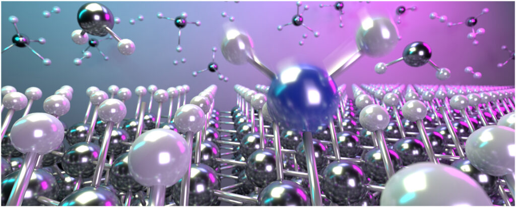 |
| Graphical Abstract: Artist impression of B incorporation during CVD growth of diamond. |
The methane concentration dependence of the plasma gas phase on surface morphology and boron incorporation in single crystal, boron-doped diamond deposition is experimentally and computationally investigated. Starting at 1%, an increase of the methane concentration results in an observable increase of the B-doping level up to 1.7×1021 cm−3, while the hole Hall carrier mobility decreases to 0.7±0.2 cm2 V−1 s−1. For B-doped SCD films grown at 1%, 2%, and 3% [CH4]/[H2], the electrical conductivity and mobility show no temperature-dependent behavior due to the metallic-like conduction mechanism occurring beyond the Mott transition. First principles calculations are used to investigate the origin of the increased boron incorporation. While the increased formation of growth centers directly related to the methane concentration does not significantly change the adsorption energy of boron at nearby sites, they dramatically increase the formation of missing H defects acting as preferential boron incorporation sites, indirectly increasing the boron incorporation. This not only indicates that the optimized methane concentration possesses a large potential for controlling the boron concentration levels in the diamond, but also enables optimization of the growth morphology. The calculations provide a route to understand impurity incorporation in diamond on a general level, of great importance for color center formation.
Permanent link to this article: https://dannyvanpoucke.be/paper_bdoping-en/
Aug 16 2020
The world of Machine-Learning (ML) and Artificial Intelligence (AI) is governed by libraries, as the implementation of a full framework from scratch requires a lot of work. ML and data-science engineers and researchers, therefore don’t generally build their own libraries. Instead they use and extend existing libraries written in python or R. One of the most popular current python ML libraries is scikit-learn. This library provides access to scores of ML-models and methods which can be combined at will via the use of a consistent global API.
However, no matter how many models there are included in such a library, chances are that a model you wish to use (or the extension you envision for an existing model) is not implemented. In such a case, you do not want to write an entire ML framework from scratch, but just create your own model and fit it into the existing framework. Within the scikit-learn framework this can be done with relative ease, as is explained in this short tutorial. As an example, I will be building a regressor class for the LS-SVM model.
Least-Squares Support Vector Machines is a type of support vector machines (SVM) initially developed some 20 years ago by researchers at the KULeuven (and is still being further developed, funded via several ERC grants). It’s a supervised learning machine learning approach in which a system of linear equations is solved using the kernel-trick.
So how does it work in practice? Assume, we have a data set of data points (xi,yi), with xi the feature vector and yi the target of the data point (or sample) i. Depending on whether you want to perform classification or regression, training the model corresponds to solving the following system of equations (represented in their matrix form as):
Classification:
Regression:
with 


Once trained, results are predicted (in case of regression) by solving the following equation:
More details on these can be found in the book of Suykens, or (if you prefer a shorter read) this paper by Dilmen.
The above model is available through the Matlab library developed by the Suykens group, and has been translated to R, but no implementation in the python scikit-learn library is available, therefore we set out to create such an implementation following the scikit-learn API. Our choice to follow the scikit-learn API is twofold: (1) we want our new class to smoothly integrate with the functionalities of the scikit-learn library (I’m building a framework for automated machine learning on this library, hence all my models need to show the same behavior and functionality) and (2) we want to be lazy and implement as little as possible.
Designing this Class, we will make full use of OOP (Similar ideas as in my fortran tutorials), inheriting behavior from scikit-learn base classes. All estimators in scikit-learn are derived from the BaseEstimator Class. The use of this class requires you to define all parameters of your class as keyword arguments in the __init__ function of your class. In return, you get the get_params and set_params methods for free.
As our goal is to create a regressor class, the class also needs to inherit from the RegressorMixin Class which provides access to the score method used by all scikit-learn regressors. With this, the initial implementation of our LS-SVM regressor class quickly takes shape:
class LSSVMRegression(BaseEstimator, RegressorMixin):
   """
   An Least Squared Support Vector Machine (LS-SVM) regression class

   Attributes:
   - gamma : the hyper-parameter (float)
   - kernel: the kernel used (string: rbf, poly, lin)
   - kernel_: the actual kernel function
   - x : the data on which the LSSVM is trained (call it support vectors)
   - y : the targets for the training data
   - coef_ : coefficents of the support vectors
   - intercept_ : intercept term
   """

   def __init__(self, gamma:float=1.0, kernel:str=None, c:float=1.0,
           d:float=2, sigma:float=1.0):
      self.gamma=gamma
      self.c=c
      self.d=d
      self.sigma=sigma
      if (kernel is None):
         self.kernel='rbf'
      else:
         self.kernel=kernel

      params=dict()
      if (kernel=='poly'):
         params['c']=c
         params['d']=d
      elif (kernel=='rbf'):
         params['sigma']=sigma

      self.kernel_=LSSVMRegression.__set_kernel(self.kernel,**params)

      self.x=None
      self.y=None
      self.coef_=None
      self.intercept_=None
All parameters have a default value in the __init__ method (and with a background in Fortran, I find it very useful to explicitly define the intended type of the parameters). Additionally, the same name is used for the attributes to which they are assigned. The kernel function is provided as a string (here we have 3 possible kernel functions: the linear (lin), the polynomial (poly), and the radial basis function (rbf) ) and linked to a function pointer via the command:
self.kernel_=LSSVMRegression.__set_kernel(self.kernel,**params)
The static private __set_kernel method returns a pointer to the correct kernel-function, which is later-on used during training and fitting. The get_params, set_params, and score methods, we get for free so no implementation is needed, but you could override them if you wish. (Note that some tutorials recommend against overriding the get_params and set_params methods.)
As our regressor class should be interchangeable with any regressor class available by scikit-learn, we look at some examples to see which method-names are being used for which purpose. Checking the LinearRegression model and the SVR model, we learn that the following methods are provided for both classes:
| method | task | LS-SVM class |
|---|---|---|
| __init__ | Initialize object of the class. | Implemented above (ourselves) |
| get_params | Get a dictionary of class parameters. | Inherited from BaseEstimator |
| set_params | Set the class parameters via a dictionary. | Inherited from BaseEstimator |
| score | Return the R2 value of the prediction. | Inherited from RegressorMixin |
| fit | Fit the model. | to do |
| predict | Predict using the fitted model. | to do |
Only the fit and predict methods are still needed to complete our LS-SVM regressor class. The implementation of the equations presented in the previous section can be done in a rather straight forward way using the numpy library.
import numpy as np

def fit(self,X:np.ndarray,y:np.ndarray):
   self.x=X
   self.y=y
   Omega=self.kernel_(self.x,self.x)
   Ones=np.array([[1]]*len(self.y))

   A_dag = np.linalg.pinv(np.block([
         [0, Ones.T ],
         [Ones, Omega + self.gamma**-1 * np.identity(len(self.y))]
         ]))
   B = np.concatenate((np.array([0]),self.y), axis=None)

   solution = np.dot(A_dag, B)
   self.intercept_ = solution[0]
   self.coef_ = solution[1:]

def predict(self,X:np.ndarray)->np.ndarray:
   Ker = self.kernel_(X,self.x)
   Y=np.dot(self.coef_,Ker.T) +self.intercept_
   return Y
Et voilà, all done. With this minimal amount of work, a new regression model is implemented and capable of interacting with the entire scikit-learn library.
The LS-SVM model has at least 1 hyperparameter: the
For the LS-SVM model, which is slightly more complex than the trivial examples found in most tutorials, you will encounter some unexpected behavior. Assume you are optimizing the hyperparameters of an LS-SVM with an rbf kernel: 
from sklearn.model_selection import GridSearchCV
...
parameters = {'kernel':('rbf'),
    'gamma':[0.001, 0.01, 0.1, 1.0, 10.0, 100.0, 1000.0],
    'sigma':[0.001, 0.01, 0.1, 1.0, 10.0, 100.0, 1000.0]}
lssvm = LSSVMRegression()
clf = GridSearchCV(lssvm, parameters)
clf.fit(X, y)
...
When you plot the quality results as a function of 

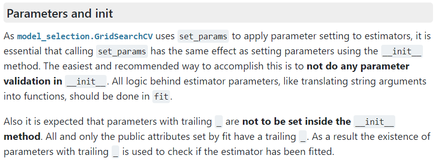
Scikit-learn manual section of parameter initialization of classes
In programming languages like C/C++ or Fortran, some may consider this as bad practice as it entirely negates the use of your constructor and splits the initialization section. For now, we will consider this a feature of the Python scripting language. This also means that getting a static class function linked to the kernel_ attribute requires us to override the get_params method (initializing attributes in a fit function is just a bridge too far 😉 ).
def set_params(self, **parameters):
   for parameter, value in parameters.items():
      setattr(self, parameter, value)

   params=dict()
   if (self.kernel=='poly'):
      params['c']=self.c
      params['d']=self.d
   elif (self.kernel=='rbf'):
      params['sigma']=self.sigma
   self.kernel_=LSSVMRegression.__set_kernel(self.kernel,**params)

   return self
For consistency the get_params method is also overridden. The resulting class is now suitable for use in combination with the rest of the scikit-learn library.
At the moment of witting no LS-SVM regressor class compatible with the scikit-learn library was available. There are some online references available to Python libraries which claim to have the LS-SVM model included, but these tend to be closed source. So instead of trying to morph these to fit my framework, I decided to use this situation as an opportunity to learn some more on the implementation of an ML model and the integration of this model in the scikit-learn framework. The resulting model is extended further to deal with the intricacies of my own framework aimed at small datasets, which is beyond the scope of the current tutorial. Since I believe the LS-SVM regressor may be of interest to other users of the scikit-learn library, you can download it from my github-page:
DISCLAIMER: Since Python codes depreciate as fast as they are written, links to the scikit-learn library documentation may be indicated as outdated by the time you read this tutorial. Check out the most recent version in that case. Normally, the changes should be sufficiently limited not to impact the conclusions drawn here. However, if you discover a code-breaking update, feel free to mention it here in the comments section.
Permanent link to this article: https://dannyvanpoucke.be/building-scikit-learn-regressor-lssvm-en/
Aug 09 2020
In the past, I discussed how to create a python script which runs your calculations in parallel. Using the multiprocessing library, you can circumvent the GIL and employing the async version of the multiprocessing functions, calculations are even performed in parallel. This works quite well, however, when using this within a python class you may run into some unexpected behaviour and errors due to the pickling performed by the multiprocessing library.
For example, if the doOneRun function is a class function defined as
class MyClass:
...
    def doOneRun(self, id:int):
       return id**3
...
and you perform some parallel calculation in another function of your class as
class MyClass:
...
    def ParallelF(self, NRuns:int):
       import multiprocessing as mp

       nproc=10
       pool=mp.Pool(processes=nprocs)
       drones=[pool.apply_async(self.doOneRun, args=(nr,)) for nr in range(NRuns)]

       for drone in drones:
           Results.collectData(drone.get())
       pool.close()
       pool.join()

...
you may run into a runtime error complaining that a function totally unrelated to the parallel work (or even to the class itself) can not be pickled. 😯
So what is going on? In the above setup, you would expect the pool.apply_async function to take just a function pointer to the doOneRun function. However, as it is provided by a the call self.doOneRun, the pool-function grabs the entire class and everything it contains, and tries to pickle it to distribute it to all the processes. In addition to the fact that such an approach is hugely inefficient, it has the side-effect that any part associated to your class needs to be pickleable, even if it is a class-function of a class used to generate an object which is just a property of the MyClass Class above.
So both for reasons of efficiency and to avoid such side-effects, it is best to make the doOneRun function independent of a class, and even placing it outside the class.
def doOneRun(id:int):
    return id**3

class MyClass:
...
    def ParallelF(self, NRuns:int):
       import multiprocessing as mp

       nproc=10
       pool=mp.Pool(processes=nprocs)
       drones=[pool.apply_async(doOneRun, args=nr) for nr in range(NRuns)]

       for drone in drones:
           Results.collectData(drone.get())
       pool.close()
       pool.join()

...
This way you avoid pickling the entire class, reducing initialization times of the processes and the unnecessary communication-overhead between processes. As a bonus, you also reduce the risk of unexpected crashes unrelated to the calculation performed.
Permanent link to this article: https://dannyvanpoucke.be/parallel-python-classes-pickle/
Aug 04 2020
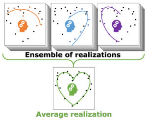
Individual model realizations may not perform that well, but the average model realization always performs very well.
Machine-Learning is up and trending. You can’t open a paper, magazine or website without someone trying to convince you their new AI-improved app/service will radically change your life. It will make the production of your company more efficient and cheaper, make costumers flock to your shop and possibly cure cancer on the side. Also in science, a lot of impressive claims are being made. General promises entail that it makes the research of interest faster, better, more efficient,… There is, however, a bit of fine print which is never explicitly mentioned: you need a LOT of data. This data is used to teach your Machine-Learning algorithm whatever it is intended to learn.
In some cases, you can get lucky, and this data is already available while in other, you still need to create it yourself. In case of computational materials science this often means performing millions upon millions of calculations to create a data set on which to train the Machine-Learning algorithm.[1] The resulting Machine-Learning model may be a thousand times faster in direct comparison, but only if you ignore the compute-time deficit you start from.
In materials science, this is not only a problem for those performing first principles modeling, but also for experimental researchers. When designing a new material, you generally do not have the resources to generate thousands or millions of samples while varying the parameters involved. Quite often you are happy if you can create even a few dozen samples. So, can this research still benefit from Machine-Learning if only very small data sets are available?
In my recent work on materials design using Machine-Learning combined with small data sets, I discuss the limitations of small data sets in the context of Machine-Learning and present a natural approach for obtaining the best possible model.[2] [3]
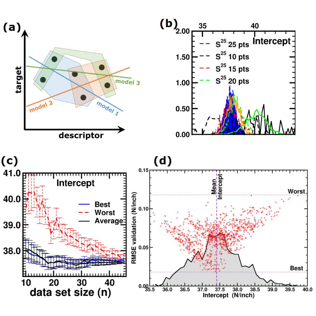
(a) Simplified representation of modeling small data sets. (b) Data set size dependence of the distribution of model coefficients. (c) Evolution of model-coefficients with data set size. (d) correlation between model coefficient value and model quality.
In Machine-Learning a data set is generally split in two parts. One part to train the model, and a second part to test the quality of the model. One of the underlying assumptions to this approach is that each subset of the data set provides an accurate representation of the “true” data/model. As a result, taking a different subset to train your data should give rise to “the same model” (ignoring small numerical fluctuations). Although this is generally true for large (and huge) data sets, for small data sets this is seldomly the case (cf. figure (a) on the side). There, the individual data points considered will have a significant impact on the final model, and different subsets give rise to very different models. Luckily the coefficients of these models still present a peaked distribution. (cf. figure (b)).
On the down side, however, if one isn’t careful in preprocessing the data set correctly, these distributions will not converge upon increasing the data set size, giving rise to erratic model behaviour.[2]
Not only the model coefficients give rise to a distribution, the same is true for the model quality. Using the same data set, but making a different split between training and test data can give rise to large differences in quality for the model instances. Interestingly, the model quality presents a strong correlation with the model coefficients, with the best quality model instances being closer to the “true” model instance. This gives rise to a simple approach: just take many train-test splittings, and select the best model. There are quite some problems with such an approach, which are discussed in the manuscript [2]. The most important one being the fact that the quality measure on a very small data set is very volatile itself. Another is the question of how many such splittings should be considered? Should it be an exhaustive search, or are any 10 random splits good enough (obviously not)? These problems are alleviated by the nice observation that “the average” model shows not the average quality or the average model coefficients, but instead it presents the quality of the best model (as well as the best model coefficients). (cf. figure (c) and (d))
This behaviour is caused by the fact that the best model instances have model coefficients which are also the average of the coefficient distributions. This observation hold for simple and complex model classes making it widely applicable. Furthermore, for model classes for which it is possible to define a single average model instance, it gives access to a very efficient predictive model as it only requires to store model coefficients for a single instance, and predictions only require a single evaluation. For models where this is not the case one can still make use of an ensemble average to benefit from the superior model quality, but at a higher computational cost.
[1] For example, take “ANI-1: an extensible neural network potential with DFT accuracy at force field computational cost“, one of the most downloaded papers of the journal of Chemical Science. The data set the authors generated to train their neural network required them to optimize 58.000 molecules using DFT calculations. Furthermore, for these molecules a total of about 17.200.000 single-point energies were calculated (again at the DFT level). I leave it to the reader to estimate the amount of calculation time this requires.
[2] “Small Data Materials Design with Machine Learning: When the Average Model Knows Best“, Danny E. P. Vanpoucke, Onno S. J. van Knippenberg, Ko Hermans, Katrien V. Bernaerts, and Siamak Mehrkanoon, J. Appl. Phys. 128, 054901 (2020)
[3] “When the average model knows best“, Savannah Mandel, AIP SciLight 7 August (2020)
Permanent link to this article: https://dannyvanpoucke.be/practical-machine-learning/
Aug 04 2020
| Authors: | Danny E. P. Vanpoucke, Onno S. J. van Knippenberg, Ko Hermans, Katrien V. Bernaerts, and Siamak Mehrkanoon |
| Journal: | Journal of Applied Physics 128, 054901 (2020) |
| doi: | 10.1063/5.0012285 |
| IF(2019): | 2.286 |
| export: | bibtex |
| pdf: | <JApplPhys> (Open Access) |
| github: | <Amadeus> |
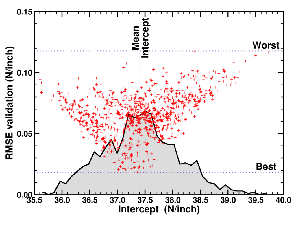 |
| Graphical Abstract: Correlation plot of the RMSE of the validation set and the intercept value for linear model instances trained on 1000 subsets of a 25 point data set. The distribution of the correlation data is indicated by the black curve. |
Machine Learning is quickly becoming an important tool in modern materials design. Where many of its successes are rooted in huge data sets, the most common applications in academic and industrial materials design deal with data sets of at best a few tens of data points. Harnessing the power of Machine Learning in this context is therefore of considerable importance. In this work, we investigate the intricacies introduced by these small data sets. We show that individual data points introduce a significant chance factor in both model training and quality measurement. This chance factor can be mitigated by the introduction of an ensemble-averaged model. This model presents the highest accuracy while at the same time it is robust with regard to changing data set size. Furthermore, as only a single model instance needs to be stored and evaluated, it provides a highly efficient model for prediction purposes, ideally suited for the practical materials scientist.
Permanent link to this article: https://dannyvanpoucke.be/paper_averagemodel-en/
Apr 22 2020
| Authors: | Danny E. P. Vanpoucke |
| Journal: | Computational Materials Science 181, 109736 (2020) |
| doi: | 10.1016/j.commatsci.2020.109736 |
| IF(2019): | 2.863 |
| export: | bibtex |
| pdf: | <ComputMaterSci> (Open Access) |
| github: | <Hive-toolbox> |
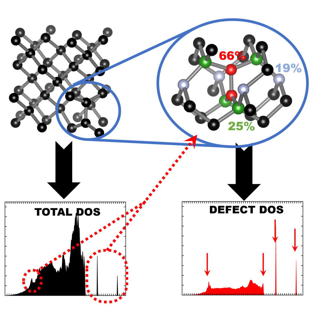 |
| Graphical Abstract: Finger printing defects in diamond through the creation of the vibrational spectrum of a defect. |
Vibrational spectroscopy techniques are some of the most-used tools for materials
characterization. Their simulation is therefore of significant interest, but commonly
performed using low cost approximate computational methods, such as force-fields.
Highly accurate quantum-mechanical methods, on the other hand are generally only used
in the context of molecules or small unit cell solids. For extended solid systems,
such as defects, the computational cost of plane wave based quantum mechanical simulations
remains prohibitive for routine calculations. In this work, we present a computational scheme
for isolating the vibrational spectrum of a defect in a solid. By quantifying the defect character
of the atom-projected vibrational spectra, the contributing atoms are identified and the strength
of their contribution determined. This method could be used to systematically improve phonon
fragment calculations. More interestingly, using the atom-projected vibrational spectra of the
defect atoms directly, it is possible to obtain a well-converged defect spectrum at lower
computational cost, which also incorporates the host-lattice interactions. Using diamond as
the host material, four point-defect test cases, each presenting a distinctly different
vibrational behaviour, are considered: a heavy substitutional dopant (Eu), two intrinsic
point-defects (neutral vacancy and split interstitial), and the negatively charged N-vacancy
center. The heavy dopant and split interstitial present localized modes at low and high
frequencies, respectively, showing little overlap with the host spectrum. In contrast, the
neutral vacancy and the N-vacancy center show a broad contribution to the upper spectral range
of the host spectrum, making them challenging to extract. Independent of the vibrational behaviour,
the main atoms contributing to the defect spectrum can be clearly identified. Recombination of
their atom-projected spectra results in the isolated spectrum of the point-defect.
Permanent link to this article: https://dannyvanpoucke.be/paper_vibrdefect-en/
Mar 24 2020
In the previous sessions of this tutorial on Object Oriented Programming in Fortran 2003, the basics of OO programming, including the implementation of constructors and destructors as well as operator overloading were covered. The resulting classes have already become quite extended (cf. github source). Although at this point it is still very clear what each part does and why certain choices were made, memory fades. One year from now, when you revisit your work, this will no longer be the case. Alternately, when sharing code, you don’t want to have to dig through every line of code to figure out how to use it. These are just some of the reasons why code documentation is important. This is a universal habit of programming which should be adopted irrespective of the programming-language and-paradigm, or size of the code base (yes, even small functions should be documented).
In Fortran, comments can be included in a very simple fashion: everything following the “!” symbol (when not used in a string) is considered a comment, and thus ignored by the compiler. This allows for quick and easy documentation of your code, and can be sufficient for single functions. However, when dealing with larger projects retaining a global overview and keeping track of interdependencies becomes harder. This is where automatic documentation generation software comes into play. These tools parse specifically formatted comments to construct API documentation and user-guides. Over the years, several useful tools have been developed for the Fortran language directly, or as a plugin/extension to a more general tool:
As you can see, there is a lot to choose from, all with their own quirks and features. One unfortunate aspect is the fact that most of these tools use different formatting conventions, so switching from one to the another is not an exercise to perform lightly. In this tutorial, the doxygen tool is used, as it provides a wide range of options, is multi-platform, supports multiple languages and multiple output formats.
As you might already expect, Object Oriented Fortran (f2003) is a bit more complicated to document than procedural Fortran, but with some ingenuity doxygen can be made to provide nice documentation even in this case.
Before you can start you will need to install doxygen:
With a nicely installed doxygen, you can make use of the GUI to setup a configuration suited to your specific needs and generate the documentation for your code automatically. For Object Oriented Fortran there are some specific settings you should consider: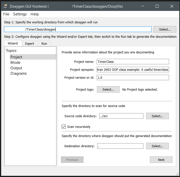
(Provides access each single configuration option to set in doxygen, so I will only highlight a few. Look through them to get a better idea of the capabilities of doxygen.)
Once you have a working configuration for doxygen, you can save this for later use. Doxygen allows you to load an old configuration file and run immediately. The configuration file for the Timer-class project is included in the docs folder, together with the pdf-latex version of the generated documentation. Doxygen generates all latex files required for generating the pdf. To generate the actual pdf, a make.bat file needs to be run (i.e. double-click the file, and watch it run) in a Windows environment.
Let us start with some basics for documenting Fortran code in a way suitable for doxygen. Since doxygen has a very extensive set of options and features, not all of them can be covered. However, the manual of more than 300 pages provides all the information you may need.
With doxygen, you are able to document more or less any part of your code: entire files, modules, functions or variables. In each case, a similar approach can be taken. Let’s consider the documentation of the TimeClass module:
[codesyntax lang=”fortran” lines=”normal” container=”div” strict=”no” title=”Documentation of the TimeClass module.” blockstate=”expanded”]
!++++++++++++++++++++++++++++++++++++++++++++++++++++++++++++++++++++++++
!> \brief The <b>TimeClass module</b> contains the
!! \link ttime TTime class\endlink used by the
!! \link timerclass::ttimer TTimer class\endlink for practical timing.
!!
!! @author  Dr. Dr. Danny E. P. Vanpoucke
!! @version 2.0-3  (upgrades deprecated timing module)
!! @date    19-03-2020
!! @copyright https://dannyvanpoucke.be
!!
!! @warning Internally, Julian Day Numbers are used to compare dates. As a
!! result, *negative* dates are not accepted. If such dates are created
!! (*e.g.*, due to a subtraction), then the date is set to zero.
!!
!! This module makes use of:
!! - nothing; this module is fully independent
!<-----------------------------------------------------------------------
module TimeClass
    implicit none
    private
[/codesyntax]
The documentation is placed in a standard single or multi-line fortran comment. In case of multi-line documentation, I have the personal habit turning it into a kind of banner starting with a “!+++++++++” line and closing with a “!<——————-” line. Such choices are your own, and are not necessary for doxygen documentation. For doxygen, a multi-line documentation block starts with “!>” and ends with “!<“ . The documentation lines in between can be indicated with “!!”. This is specifically for fortran documentation in doxygen. C/C++ and other languages will have slightly different conventions, related to their comment section conventions.
In the block above, you immediately see certain words are preceded by an “@”-symbol or a “\”, this indicates these are special keywords. Both the “@” and “\” can be used interchangeably for most keywords, the preference is again personal taste. Furthermore, doxygen supports both html and markdown notation for formatting, providing a lot of flexibility. The multi-line documentation is placed before the object being documented (here an entire module).
Some keywords:
[codesyntax lang=”fortran” lines=”normal” container=”div” capitalize=”no” strict=”no” title=”Documentation of a function” blockstate=”expanded”]
!++++++++++++++++++++++++++++++++++++++++++++++
!>\brief Function to subtract two \link ttime TTime\endlink instance
!! via the "-" operator. This is the function
!! performing the actual operator overloading.
!!
!! \b usage:
!! \code{.f03}
!! Total = this - that
!! \endcode
!! This line also calls the \link copy assignment operator\endlink.
!!
!! \note The result should remain a positive number.
!!
!! @param[in] this The \link ttime TTime\endlink instance before
!!                 the "-" operator.
!! @param[in] that The \link ttime TTime\endlink instance after
!!                 the "-" operator.
!! \return Total The \link ttime TTime\endlink instance representing
!!               the difference.
!<---------------------------------------------
    pure function subtract(this,that) Result(Total)
        class(TTime), intent(in) :: this, that
        Type(TTime) :: total
[/codesyntax]
When documenting functions and subroutines there are some addition must-have keywords.
With the knowledge of the previous section, it is relatively easy to document most fortran code. Also the type of object orientation available in fortran 95, in which a fortran module is refurbished as a class. True fortran classes in contrast tend to give a few unexpected issues to deal with. Lets have a look at the documentation of the TTime class of the TimeClass module:
[codesyntax lang=”fortran” lines=”normal” container=”div” capitalize=”no” strict=”no” title=”Documentation of a fortran class definition” blockstate=”expanded”]
!+++++++++++++++++++++++++++++++++++++++
!> @class ttime
!! \brief The TTime class contains all time functionality
!! with regard to a single time stamp.
!<-------------------------------------
    type, public :: TTime
      private
        integer :: year    !< @private The year
        integer :: month   !< @private The month (as integer).
        ...
    contains
      private
        procedure, pass(this),public :: SetTime       !<          @copydoc timeclass::settime
        procedure, pass(this)        :: CalculateJDN  !< @private @copydoc timeclass::calculatejdn
        procedure, pass(this)        :: SetJDN        !< @private @copydoc timeclass::setjdn
        ...
        procedure, pass(this)        :: copy          !< @private @copydoc timeclass::copy
        ...
        generic, public :: assignment(=) => copy      !<          @copydoc timeclass::copy
        !> @{ @protected
        final :: destructor !< @copydoc timeclass::destructor
        !> @}
    end type TTime

    ! This is the only way a constructor can be created,
    ! as no "initial" exists, emulates the C++ constructor behavior
    interface TTime
        module procedure constructor
    end interface TTime
[/codesyntax]
To make sure doxygen generates a class-like documentation for our fortran class, it needs to be told it is a class. This can be done by documenting the class itself and using the keyword @class nameclass, with nameclass the name doxygen will use for this class (so you can choose something different from the actual class name). Unfortunately, doxygen will call this a “module” in the documentation (just poor luck in nomenclature). On the module page for the ttime class a listing is provided of all elements given in the class definition. The documentation added to each member (e.g.,:
[codesyntax lang=”fortran” lines=”normal” container=”div” capitalize=”no” strict=”no”]
integer :: year !< @private The year
[/codesyntax]
is shown as “\brief” documentation. By default all members of our function are considered as public. Adding the @private, @public, or @protected keyword instructs doxygen explicitly to consider these members as private, public or protected. (I used protected in the ttime code not as it should be used in fortran, but as a means of indicating the special status of the final subroutine (i.e. protected in a C++ way).)
However, there seems to be something strange going on. When following the links in the documentation, we do not end up with the documentation provided for the functions/subroutines in the body of our timeclass module. Doxygen seems to consider these two distinct things. The easiest way to link the correct information is by using the keyword @copydoc functionreference . The documentation is (according to doxygen) still for two distinctly different objects, however, this time they have the exact same documentation (unless you add more text on the member documentation line). In this context, it interesting to know there is also @copybrief and @copydetails which can be used to only copy the brief/details section.
In this example, the constructor interface is not documented, as this created confusion in the final documentation since doxygen created a second ttime module/object linked to this interface. However, not documenting this specific instance of the constructor does not create such a large issue, as the module(the fortran module) function itself is documented already.
Documenting fortran classes can be done quite nicely with doxygen. It provides various modes of output: from a fully working website with in-site search engine to a hyperlinked pdf or RTF document. The flexibility and large number of options may be a bit daunting at first, but you can start simple, and work your way up.
As Fortran is supported as an extension, you will need to play around with the various options to find which combination gives the effect you intended. This is an aspect present in all automated code documentation generation tools, since object oriented Fortran is not that widely used. Nonetheless, doxygen provides a very powerful tool worth your time and effort.
Permanent link to this article: https://dannyvanpoucke.be/oop-fortran-tut6-en/
Mar 14 2020
Last Wednesday, the 25th edition of the Hasselt Diamond workshop started. The central topic of this celebratory edition was focused on surfaces, perfectly suited to present some of my more recent diamond based work.[1][2] Just as the previous years, the program was packed with interesting talks on anything diamond. Phosphorous doped diamond seemed to be the “new thing” this year, but I could be biased, as I was speaking on phosphorous adsorption myself. Due to a cancellation, I found myself being asked on Monday afternoon to present my work as a talk 😎 , on Wednesday morning 😯 . Because I had been a bit too ambitious in my conference abstract, this talk ended up being nicely complementary to my poster.
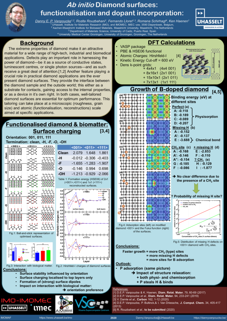
Unfortunately, this celebratory edition also fell victim to the COVID-19 crisis. In addition to being the most popular conversation topic—a close second to diamond research—, it also had a very real impact on the conference itself. The COVID-19 crisis resulted in a drop of attendance from 238 people in 2019 to 143 this year. In addition, the quickly changing situation worldwide lead to last minute cancellations due to travel restrictions. On Thursday evening, the conference site went into lock down. Furthermore, that evening, the Belgian federal government also decided that schools and higher education should be closed, as well as pubs and restaurants, until April 3rd. There was also the urgent request for people to work from home as much as possible. (Consider this a good example of acting NOW aimed at saving people.)
Consider this computational scientist in lock down in his home lab until further notice.
Permanent link to this article: https://dannyvanpoucke.be/sbdd-25-aka-the-covid19-edition/
Feb 25 2020
| Authors: | Jules Stouten, Danny E. P. Vanpoucke, Guy Van Assche, and Katrien V. Bernaerts |
| Journal: | Macromolecules 53(4), 1388-1404 (2020) |
| doi: | 10.1021/acs.macromol.9b02659 |
| IF(2019): | 5.918 |
| export: | bibtex |
| pdf: | <Macromolecules> (Open Access) |
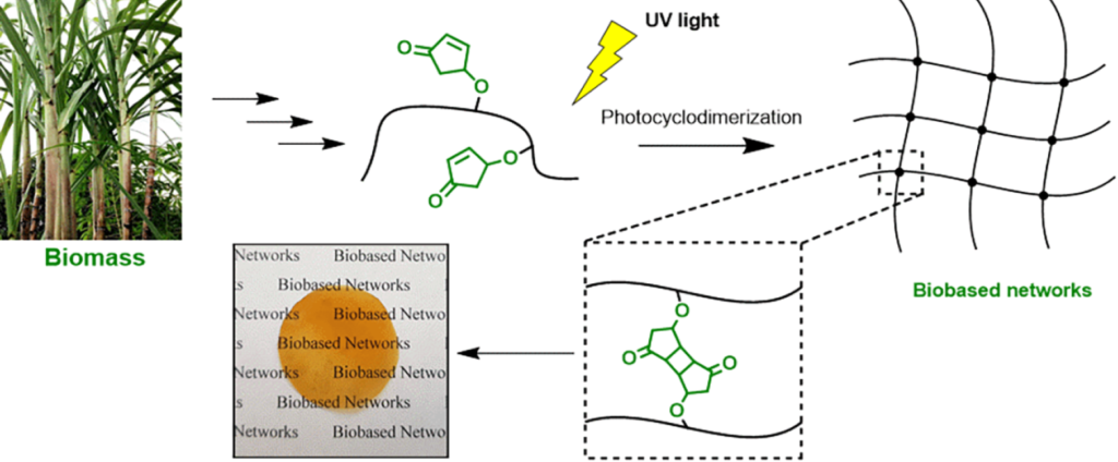 |
| Graphical Abstract: The formation of biobased polyacrylates. |
The controlled polymerization of a new biobased monomer, 4-oxocyclopent-2-en-1-yl acrylate (4CPA), was
established via reversible addition−fragmentation chain transfer (RAFT) (co)polymerization to yield polymers bearing pendent cyclopentenone units. 4CPA contains two reactive functionalities, namely, a vinyl group and an internal double bond, and is an unsymmetrical monomer. Therefore, competition between the internal double bond and the vinyl group eventually leads to gel formation. With RAFT polymerization, when aiming for a degree of polymerization (DP) of 100, maximum 4CPA conversions of the vinyl group between 19.0 and 45.2% were obtained without gel formation or extensive broadening of the dispersity. When the same conditions were applied in the copolymerization of 4CPA with lauryl acrylate (LA), methyl acrylate (MA), and isobornyl acrylate, 4CPA conversions of the vinyl group between 63 and 95% were reached. The additional functionality of 4CPA in copolymers was demonstrated by model studies with 4-oxocyclopent-2-en-1-yl acetate (1), which readily dimerized under UV light via [2 + 2] photocyclodimerization. First-principles quantum mechanical simulations supported the experimental observations made in NMR. Based on the calculated energetics and chemical shifts, a mixture of head-to-head and head-to-tail dimers of (1) were identified. Using the dimerization mechanism, solvent-cast LA and MA copolymers containing 30 mol % 4CPA were cross-linked under UV light to obtain thin films. The cross-linked films were characterized by dynamic scanning calorimetry, dynamic mechanical analysis, IR, and swelling experiments. This is the first case where 4CPA is described as a monomer for functional biobased polymers that can undergo additional UV curing via photodimerization.
Permanent link to this article: https://dannyvanpoucke.be/paper_nmrjules-en/


