Tag: diamond

Revisiting the Neutral C-Vacancy in Diamond: Localization of Electrons through DFT+U

Authors: Danny E. P. Vanpoucke and Ken Haenen
Journal: Diam. Relat. Mater 79, 60-69 (2017)
doi: 10.1016/j.diamond.2017.08.009
IF(2017): 2.232
export: bibtex
pdf: <DiamRelatMater>


Combining a scan over possible values for U and J with reference electronic structures obtained using the hybrid functional HSE06, DFT+U can be fit to provide hybrid functional quality electronic structures at the cost of DFT calculations.
Graphical Abstract: Combining a scan over possible values for U and J with reference electronic structures obtained using the hybrid functional HSE06, DFT+U can be fit to provide hybrid functional quality electronic structures at the cost of DFT calculations.

Abstract

The neutral C-vacancy is investigated using density functional theory calculations. We show that local functionals, such as PBE, can predict the correct stability order of the different spin states, and that the success of this prediction is related to the accurate description of the local magnetic configuration. Despite the correct prediction of the stability order, the PBE functional still fails predicting the defect states correctly. Introduction of a fraction of exact exchange, as is done in hybrid functionals such as HSE06, remedies this failure, but at a steep computational cost. Since the defect states are strongly localized, the introduction of additional on site Coulomb and exchange interactions, through the DFT+U method, is shown to resolve the failure as well, but at a much lower computational cost. In this work, we present optimized U and J parameters for DFT+U calculations, allowing for the accurate prediction of defect states in defective
diamond. Using the PBE optimized atomic structure and the HSE06 optimized electronic structure as reference, a pair of on-site Coulomb and exchange parameters (U,J) are fitted for DFT+U studies of defects in diamond.

Related:

Poster-presentation: here

DFT+U series (varying J) for a specific spin state of the C-vacancy defect.

DFT+U series (varying J) for a specific spin state of the C-vacancy defect.

Bachelor Projects Completed: 2 new computational materials scientists initialised

The black arts of computational materials science.

Black arts of computational materials science.

Just over half a year ago, I mentioned that I presented two computational materials science related projects for the third bachelor physics students at the UHasselt. Both projects ended up being chosen by a bachelor student, so I had the pleasure of guiding two eager young minds in their first steps into the world of computational materials science. They worked very hard, cursed their machine or code (as any good computational scientist should do once in a while, just to make sure that he/she is still at the forefront of science) and survived. They actually did quite a bit more than “just surviving”, they grew as scientists and they grew in self-confidence…given time I believe they may even thrive within this field of research.

One week ago, they presented their results in a final presentation for their classmates and supervisors. The self-confidence of Giel, and the clarity of his story was impressive. Giel has a knack for storytelling in (a true Pan Narrans as Terry Pratchett would praise him). His report included an introduction to various topics of solid state physics and computational materials science in which you never notice how complicated the topic actually is. He just takes you along for the ride, and the story unfolds in a very natural fashion. This shows how well he understands what he is writing about.

This, in no way means his project was simple or easy. Quite soon, at the start of his project Giel actually ran into a previously unknown VASP bug. He had to play with spin-configurations of defects and of course bumped into a hand full of rookie mistakes which he only made once *thumbs-up*. (I could have warned him for them, but I believe people learn more if they bump their heads themselves. This project provided the perfect opportunity to do so in a safe environment. 😎 )  His end report was impressive and his results on the Ge-defect in diamond are of very good quality.

The second project was brought to a successful completion by Asja. This very eager student actually had to learn how to program in fortran before he could even start. He had to implement code to calculate partial phonon densities with the existing HIVE code. Along the way he also discovered some minor bugs (Thank you very much 🙂  ) and crashed into a rather unexpected hard one near the end of the project. For some time, things looked very bleak indeed: the partial density of equivalent atoms was different, and the sum of all partial densities did not sum to the total density. As a result there grew some doubts if it would be possible to even fulfill the goal of the project. Luckily, Asja never gave up and stayed positive, and after half a day of debugging on my part the culprit was found (in my part of the code as well). Fixing this he quickly started torturing his own laptop calculating partial phonon densities of state for Metal-organic frameworks and later-on also the Ge-defect in diamond, with data provided by Giel. Also these results are very promising and will require some further digging, but they will definitely be very interesting.

For me, it has been an interesting experience, and I count myself lucky with these two brave and very committed students. I wish them all the best of luck for the future, and maybe we meet again.

VSC-user day 2017: The Poster Edition

Last Friday, the HPC infrastructure in Flanders got celebrated by the VSC user day. Being one of the Tier-1 supercomputer users at UHasselt, I was asked if I could present a poster at the meeting, showcasing the things I do here. Although I was very interested in this event, educational obligations (the presentations of the bachelor projects, on which I will post later) prevented me from attending the meeting.

As means of a compromise, I created a poster for the meeting which Geert Jan Bex, our local VSC/HPC support team, would be so nice to put up at the event. The poster session was preceded by a set of 1-minute presentations of the posters, for which a slide had to be made. As I could not be physically present, I provided the organizers a slide which contained a short description that could be used as the 1-minute presentation. Unfortunately, things got a little mixed up, as Geert Jan accidentally printed this slide as the poster (which gave rise to some difficulties in the printing process 🙄 ). So for those who might have had an interest in the actual poster, let me put it up here:

This poster presents my work on linker functionalisation of the MIL-47, which got recently published in the Journal of physical chemistry C, and the diamond work on the C-vacancy, which is currently submitted. Clicking on the poster above will provide you the full size image. The 1-minute slide presentation, which erroneously got printed as poster:

VASP tutor: Structure optimization through Equation-of-State fitting

Materials properties, such as the electronic structure, depend on the atomic structure of a material. For this reason it is important to optimize the atomic structure of the material you are investigating. Generally you want your system to be in the global ground state, which, for some systems, can be very hard to find. This can be due to large barriers between different conformers, making it easy to get stuck in a local minimum. However, a very shallow energy surface will be problematic as well, since optimization algorithms can get stuck wandering these plains forever, hopping between different local minima (Metal-Organic Frameworks (MOFs) and other porous materials like Covalent-Organic Frameworks and Zeolites are nice examples).

VASP, as well as other ab initio software, provides multiple settings and possibilities to perform structure optimization. Let’s give a small overview, which I also present in my general VASP introductory tutorial, in order of increasing workload on the user:

  1. Experimental Structure: This the most lazy option, as it entails just taking an experimentally obtained structure and not optimizing it at all. This should be avoided unless you have a very specific reason why you want to use specifically this geometry. (In this regard, Force-Field optimized structures fall into the same category.)
  2. Simple VASP Optimization: You can let VASP do the heavy lifting. There are several parameters which help with this task.
    1. IBRION = 1 (RMM-DIIS, good close to a minimum), 2 (conjugate gradient, safe for difficult problems, should always work), 3 (damped molecular dynamics, useful if you start from a bad initial guess) The IBRION tag determines how ions are moved during relaxation.
    2. ISIF = 2 (Ions only, fixed shape and volume), 4 (Ions and cell shape, fixed volume), 3 (ions, shape and volume relaxed) The ISIF tag determines how the stress tensor is calculated, and which degrees of freedom can change during a relaxation.
    3. ENCUT = max(ENMAX)x1.3  To reduce Pulay stresses, it is advised to increase the basis set to 1.3x the default value, which is the largest ENMAX value for the atoms used in your system.
  1. Volume Scan (Quick and dirty): For many systems, especially simple systems, the internal coordinates of the ions are often well represented in available structure files. The main parameter which needs optimization is the lattice parameter. This is also often the main change if different functional are used. In a quick and dirty volume scan, one performs a set of static calculations, only the volume of the cell is changed. The shape of the cell and the internal atom coordinates are kept fixed. Fitting a polynomial to the resulting Energy-Volume data can then be used to obtain the optimum volume. This option is mainly useful as an initial guess and should either be followed by option 2, or improved to option 4.
  2. Equation of state fitting to fixed volume optimized structures: This approach is the most accurate (and expensive) method. Because you make use of fixed volume optimizations (ISIF = 4), the errors due to Pulay stresses are removed. They are still present for each separate fixed volume calculation, but the equation of state fit will average out the basis-set incompleteness, as long as you take a large enough volume range: 5-10%. Note that the 5-10% volume range is generally true for small systems. In case of porous materials, like MOFs, ±4% can cover a large volume range of over 100 Å3. Below you can see a pseudo-code algorithm for this setup. Note that the relaxation part is split up in several consecutive relaxations. This is done to further reduce basis-set incompleteness errors. Although the cell volume does not change, the shape does, and the original sphere of G-vectors is transformed into an ellipse. At each restart this is corrected to again give a sphere of G-vectors. For many systems the effect may be very small, but this is not always the case, and it can be recognized as jumps in the energy going from one relaxation calculation to the next. The convergence is set the usual way for a relaxation in VASP (EDIFF and EDIFFG parameters) and a threshold in the number of ionic steps should be set as well (5-10 for normal systems is reasonable, while for porous/flexible materials you may prefer a higher value). There exist several possible equations-of-state which can be used for the fit of the E(V) data. The EOSfit option of HIVE-4 implements 3:
    1. Birch-Murnaghan third order isothermal equation of state
    2. Murnaghan equation of state
    3. Rose-Vinet equation of state (very well suited for (flexible) MOFs)

    Using the obtained equilibrium volume a final round of fixed volume relaxations should be done to get the fully optimized structure.

For (set of Volumes: equilibrium volume ±5%){
	Step 1          : Fixed Volume relaxation
	(IBRION = 2, ISIF=4, ENCUT = 1.3x ENMAX, LCHARG=.TRUE., NSW=100)
	Step 2→n-1: Second and following fixed Volume relaxation (until a threshold is crossed and the structure is relaxed in fewer than N ionic steps) (IBRION = 2, ISIF=4, ENCUT = 1.3x ENMAX, ICHARG=1, LCHARG=.TRUE., NSW=100) 
	Step n : Static calculation (IBRION = -1, no ISIF parameter, ICHARG=1, ENCUT = 1.3x ENMAX, ICHARG=1, LCHARG=.TRUE., NSW=0) 
} 
Fit Volume-Energy to Equation of State.
Fixed volume relaxation at equilibrium volume. (With continuations if too many ionic steps are required.) 
Static calculation at equilibrium volume
EOS-fitting Diamond and Graphite

Top-left: Volume scan of Diamond. Top-right: comparison of volume scan and equation of state fitting to fixed volume optimizations, showing the role of van der Waals interactions. Bottom: Inter-layer binding in graphite for different functionals.

Some examples

Let us start with a simple and well behaved system: Diamond. This material has a very simple internal structure. As a result, the internal coordinates should not be expected to change with reasonable volume variations. As such, a simple volume scan (option 3), will allow for a good estimate of the equilibrium volume. The obtained bulk modulus is off by about 2% which is very good.

Switching to graphite, makes things a lot more interesting. A simple volume scan gives an equilibrium volume which is a serious overestimation of the experimental volume (which is about 35 Å3), mainly due to the overestimation of the c-axis. The bulk modulus is calculated to be 233 GPa a factor 7 too large. Allowing the structure to relax at fixed volume changes the picture dramatically. The bulk modulus drops by 2 orders of magnitude (now it is about 24x too small) and the equilibrium volume becomes even larger. We are facing a serious problem for this system. The origin lies in the van der Waals interactions. These weak forces are not included in standard DFT, as a result, the distance between the graphene sheets in graphite is gravely overestimated. Luckily several schemes exist to include these van der Waals forces, the Grimme D3 corrections are one of them. Including these the correct behavior of graphite can be predicted using an equation of state fit to fixed volume optimizations.(Note that the energy curve was shifted upward to make the data-point at 41 Å3 coincide with that of the other calculations.) In this case the equilibrium volume is correctly estimated to be about 35 Å3 and the bulk modulus is 28.9 GPa, a mere 15% off from the experimental one, which is near perfect compared to the standard DFT values we had before.

In case of graphite, the simple volume scan approach can also be used for something else. As this approach is well suited to check the behaviour of 1 single internal parameter, we use it to investigate the inter-layer interaction. Keeping the a and b lattice vectors fixed, the c-lattice vector is scanned. Interestingly the LDA functional, which is known to overbind, finds the experimental lattice spacing, while both PBE and HSE06 overestimate it significantly. Introducing D3 corrections for these functionals fixes the problem, and give a stronger binding than LDA.

EOS-fitting for MIL53-MOFs

Comparison of a volume scan and an EOS-fit to fixed volume optimizations for a Metal-Organic Framework with MIL53/47 topology.

We just saw that for simple systems, the simple volume scan can already be too simple. For more complex systems like MOFs, similar problems can be seen. The simple volume scan, as for graphite gives a too sharp potential (with a very large bulk modulus). In addition, internal reordering of the atoms gives rise to very large changes in the energy, and the equilibrium volume can move quite a lot. It even depends on the spin-configuration.

In conclusion: the safest way to get a good equilibrium volume is unfortunately also the most expensive way. By means of an equation of state fit to a set of fixed volume structure optimizations the ground state (experimental) equilibrium volume can be found. As a bonus, the bulk modulus is obtained as well.

Folding Phonons

Game-diamondsAbout a year ago, I discussed the possibility of calculating phonons (the collective vibration of atoms) in the entire Brillouin zone for Metal-Organic Frameworks. Now, one year later, I return to this topic, but this time the subject matter is diamond. In contrast to Metal-Organic Frameworks, the unit-cell of diamond is very small (only 2 atoms). Because a phonon spectrum is calculated through the gradients of forces felt by one atom due to all other atoms, it is clear that within one diamond unit-cell these forces will not be converged. As such, a supercell will be needed to make sure the contribution, due to the most distant atoms, to the experienced forces, are negligible.

Using such a supercell has the unfortunate drawback that the dynamical matrix (which is 3N \times 3N, for N atoms) explodes in size, and, more importantly, that the number of eigenvalues, or phonon-frequencies also increases (3N) where we only want to have 6 frequencies ( 3 \times 2 atoms) for diamond. For an M \times M \times M supercell we end up with 24M^3 -6  additional phonon bands which are the result of band-folding. Or put differently, 24M^3 -6 phonon bands coming from the other unit-cells in the supercell. This is not a problem when calculating the phonon density of states. It is, however, a problem when one is interested in the phonon band structure.

The phonon spectrum at a specific q-point in the first Brillouin zone is given by the square root of the eigenvalues of the dynamical matrix of the system. For simplicity, we first assume a finite system of n atoms (a molecule). In that case, the first Brillouin zone is reduced to a single point q=(0,0,0) and the dynamical matrix looks more or less like the hessian:
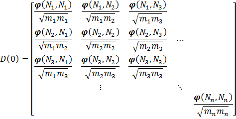
With \varphi (N_a,N_b) = [\varphi_{i,j}(N_a , N_b)] 3 \times 3 matrices \varphi_{i,j}(N_a,N_b)=\frac{\partial^2\varphi}{\partial x_i(N_a) \partial x_j(N_b)} = - \frac{\partial F_i (N_a)}{\partial x_j (N_b)}  with i, j = x, y, z. Or in words, \varphi_{i,j}(N_a , N_b) represents the derivative of the force felt by atom N_a due to the displacement of atom N_b. Due to Newton’s second law, the dynamical matrix is expected to be symmetric.

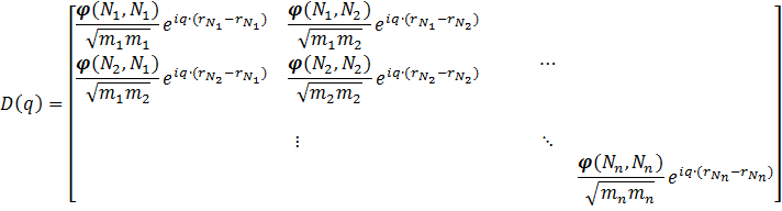
When the system under study is no longer a molecule or a finite cluster, but an infinite solid, things get a bit more complicated. For such a solid, we only consider the symmetry in-equivalent atoms (in practice this is often a unit-cell). Because the first Brillouin zone is no longer a single point, one needs to sample multiple different points to get the phonon density-of-states. The role of the q-point is introduced in the dynamical matrix through a factor e^{iq \cdot (r_{N_a} - r_{N_b}) }, creating a dynamical matrix for a single unit-cell containing n atoms:

Because a real solid contains more than a single unit-cell, one should also take into account the interactions of the atoms of one unit-cell with those of all other unit-cells in the system, and as such the dynamical matrix becomes a sum of matrices like the one above:

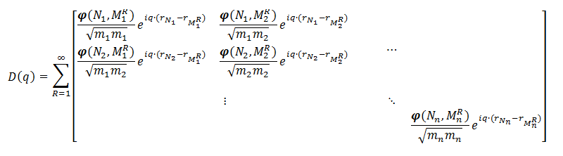
Where the sum runs over all unit-cells in the system, and Ni indicates an atom in a specific reference unit-cell, and MRi  an atom in the Rth unit-cells, for which we give index 1 to the reference unit-cell. As the forces decay with the distance between the atoms, the infinite sum can be truncated. For a Metal-Organic Framework a unit-cell will quite often suffice. For diamond, however, a larger cell is needed.

An interesting aspect to the dynamical matrix above is that all matrix-elements for a sum over n unit-cells are also present in a single dynamical matrix for a supercell containing these n unit-cells. It becomes even more interesting if one notices that due to translational symmetry one does not need to calculate all elements of the entire supercell dynamical matrix to construct the full supercell dynamical matrix.

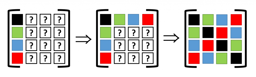
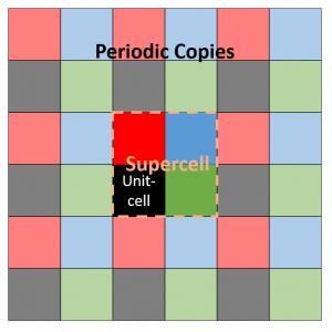
Assume a 2D 2×2 supercell with only a single atom present, which we represent as in the figure on the right. A single periodic copy of the supercell is added in each direction. The dynamical matrix for the supercell can now be constructed as follows: Calculate the elements of the first column (i.e. the gradient of the force felt by the atom in the reference unit-cell, in black, due to the atoms in each of the unit-cells in the supercell). Due to Newton’s third law (action = reaction), this first column and row will have the same elements (middle panel).

Translational symmetry on the other hand will allow us to determine all other elements. The most simple are the diagonal elements, which represent the self-interaction (so all are black squares). The other you can just as easily determine by looking at the schematic representation of the supercell under periodic boundary conditions. For example, to find the derivative of the force on the second cell (=second column, green square in supercell) due to the third cell (third row, blue square in supercell), we look at the square in the same relative position of the blue square to the green square, when starting from the black square: which is the red square (If you read this a couple of times it will start to make sense). Like this, the dynamical matrix of the entire supercell can be constructed.

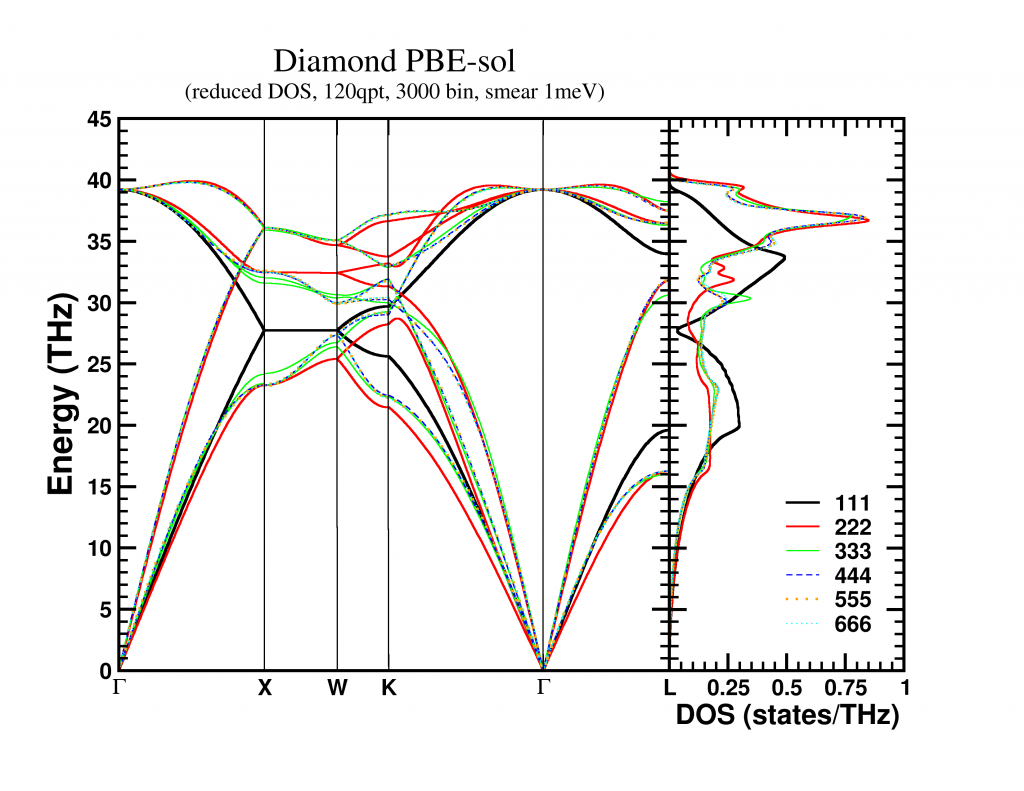
This final supercell dynamical matrix can, with the same ease, be folded back into the sum of unit-cell dynamical matrices (it becomes an extended lookup-table). The resulting unit-cell dynamical matrix can then be used to create a band structure, which in my case was nicely converged for a 4x4x4 supercell. The bandstructure along high symmetry lines is shown below, but remember that these are actually 3D surfaces. A nice video of the evolution of the first acoustic band (i.e. lowest band) as function of its energy can be found here.

The phonon density of states can also be obtained in two ways, which should, in contrast to the band structure, give the exact same result: (for an M \times M \times M supercell with n atoms per unit-cell)

  1. Generate the density of states for the supercell and corresponding Brillouin zone. This has the advantage that the smaller Brillouin zone can be sampled with fewer q-points, as each q-point acts as M3 q-points in a unit-cell-approach. The drawback here is the fact that for each q-point a (3nM3)x(3nM3) dynamical matrix needs to be solved. This solution scales approximately as O(N3) ~ (3nM3)3 =(3n)3M9. Using linear algebra packages such as LAPACK, this may be done slightly more efficient (but you will not get O(N2) for example).
  2. Generate the density of states for the unit-cell and corresponding Brillouin zone. In this approach, the dynamical matrix to solve is more complex to construct (due to the sum which needs to be taken) but much smaller: 3nx3n. However to get the same q-point density, you will need to calculate M3 times as many q-points as for the supercell.

In the end, the choice will be based on whether you are limited by the accessible memory (when running a 32-bit application, the number of q-point will be detrimental) or CPU-time (solving the dynamical matrix quickly becomes very expensive).


SBDD XXI

SBDD XXI logoToday was the first day of the three-day long diamond conference at the university of Hasselt. And although this sounds as-if it is a mere small-scale local conference, it is actually one of the two main international conferences in the field. The Surface and Bulk Defects in Diamond (SBDD) workshop grew in twenty years from a small event with only a few dozen participants to the current event with over 200 participants. As such, it is the place to be, for one as me, who is dipping into a new field of materials.

One thing that already became quite clear today, is the fact that there are many opportunities in this field for the computational materials scientist, as the large majority of the researchers are experimentalists. Of the >120 posters presented, I have only discovered about 5 theoretical ones. Having had very nice chats with their presenters I already learned a lot of what I will have to keep in mind when studying diamond. But so far, I have not come across any issues that are impossible to resolve, which is good news :-).