Tag: scientific programming

Defensive Programming and Debugging

Last few months, I finally was able to remove something which had been lingering on my to-do list for a very long time: studying debugging in Fortran. Although I have been programming in Fortran for over a decade, and getting quite good at it, especially in the more exotic aspects such as OO-programming, I never got around to learning how to use decent debugging tools. The fact that I am using Fortran was the main contributing factor. Unlike other languages, everything you want to do in Fortran beyond number-crunching in procedural code has very little documentation (e.g., easy dll’s for objects), is not natively supported (e.g., find a good IDE for fortran, which also supports modern aspects like OO, there are only very few who attempt), or you are just the first to try it (e.g., fortran programs for android :o, definitely on my to-do list). In a long bygone past I did some debugging in Delphi (for my STM program) as the debugger was nicely integrated in the IDE. However, for Fortran I started programming without an IDE and as such did my initial debugging with well placed write statements. And I am a bit ashamed to say, I’m still doing it this way, because it can be rather efficient for a large code spread over dozens of files with hundreds of procedures.

However, I am trying to repent for my sins. A central point in this penance was enlisting for the online MOOC  “Defensive Programming and Debugging“. Five weeks of intense study followed, in which I was forced to use command line gdb and valgrind. During these five weeks I also sharpened my skills at identifying possible sources of bugs (and found some unintentional bugs in the course…but that is just me). Five weeks of hard study, and taking tests, I successfully finished the course, earning my certificate as defensive programmer and debugger. (In contrast to my sometimes offensive programming and debugging skills before 😉 .)

A Spectre and Meltdown victim: VASP

Over the last weekend, two serious cyber security issues were hot news: Meltdown and Spectre [more links, and links](not to be mistaken for a title of a bond-movie). As a result, also academic HPC centers went into overdrive installing patches as fast as possible. The news of the two security issues went hand-in-hand with quite a few belittling comments toward the chip-designers ignoring the fact that no-one (including those complaining now) discovered the problem for over decade. Of course there was also the usual scare-mongering (cyber-criminals will hack our devices by next Monday, because hacks using these bugs are now immediately becoming their default tools etc.) typical since the beginning of the  21st century…but now it is time to return back to reality.

One of the big users on scientific HPC installations is the VASP program(an example), aimed at the quantum mechanical simulation of materials, and a program central to my own work. Due to an serendipitous coincidence of a annoyingly hard to converge job I had the opportunity to see the impact of the Meltdown and Spectre patches on the performance of VASP: 16% performance loss (within the range of the expected 10-50% performance loss for high performance applications [1][2][3]).

The case:

  • large HSE06 calculation of a 71 atom defective ZnO supercell.
  • 14 irreducible k-points (no reduction of the Hartree-Fock k-points)
  • 14 nodes of 24 cores, with KPAR=14, and NPAR=1 (I know NPAR=24 is the recommended option)

The calculation took several runs of about 10 electronic steps (of each about 5-6 h wall-time, about 2.54 years of CPU-time per run) . The relative average time is shown below (error-bars are the standard deviation of the times within a single run). As the final step takes about 50% longer it is treated separately. As you can see, the variation in time between different electronic steps is rather small (even running on a different cluster only changes the time by a few %). The impact of the Meltdown/Spectre patch gives a significant impact.

Impact of Meltdown/Spectre patch on VASP performance

Impact of Meltdown/Spectre patch on VASP performance for a 336 core MPI job.


The HPC team is currently looking into possible workarounds that could (partially) alleviate the problem. VASP itself is rather little I/O intensive, and a first check by the HPC team points toward MPI (the parallelisation framework required for multi-node jobs) being ‘a’ if not ‘the’ culprit. This means that also an impact on other multi-node programs is to be expected. On the bright side, finding a workaround for MPI would be beneficial for all of them as well.

So far, tests I performed with the HPC team not shown any improvements (recompiling VASP didn’t help, nor an MPI related fix). Let’s keep our fingers crossed, and hope the future brings insight and a solution.


Exa-scale computing future in Europe?

As a computational materials scientist with a main research interest in the ab initio simulation of materials, computational resources are the life-blood of my research. Over the last decade, I have seen my resource usage grow from less than 100.000 CPU hours per year to several million CPU-hours per year. To satisfy this need for computational resources I have to make use of HPC facilities, like the TIER-2 machines available at the Flemish universities and the Flemish TIER-1 supercomputer, currently hosted at KU Leuven. At the international level, computational scientists have access to so called TIER-0 machines, something I no doubt will make use of in the future. Before I continue, let me first explain a little what this TIER-X business actually means.

The TIER-X notation is used to give an indication of the size of the computer/supercomputer indicated. There are 4 sizes:

  •  TIER-3: This is your personal computer(laptop/desktop) or even a small local cluster of a research group. It can contain from one (desktop) up to a few hundred CPU’s (local cluster). Within materials research, this is sufficient for quite a few tasks: post-processing of data, simple force-field based calculations, or even small quantum chemical or solid state calculations. A large fraction of the work during my first Ph.D. was performed on the local cluster of the CMS.
  • TIER-2: This is a supercomputer hosted by an institute or university. It generally contains over 1000 CPUs and has a peak performance of >10 TFLOPS (1012 Floating Point Operations Per Second, compare this to 1-50×10FLOPS or 1-25 GFLOPS of an average personal computer). The TIER-2 facilities of the VUB and UAntwerp both have a peak performance of about 75TFLOPS , while the machines at Ghent University and the KU Leuven/Uhasselt facilities both have a peak performance of about 230 TFLOPS. Using these machines I was able to perform the calculations necessary for my study of dopant elements in cerates (and obtain my second Ph.D.).
  • TIER-1: Moving up one more step, there are the national/regional supercomputers. These generally contain over 10.000 CPUs and have a peak performance of over 100 TFLOPS. In Flanders the Flemish Supercomputer Center (VSC) manages the TIER-1 machine (which is being funded by the 5 Flemish universities). The first TIER-1 machine was hosted at Ghent University, while the second and current one is hosted at KU Leuven, an has a peak performance of 623 TFLOPS (more than all TIER-2 machines combined), and cost about 5.5 Million € (one of the reasons it is a regional machine). Over the last 5 years, I was granted over 10 Million hours of CPU time, sufficient for my study of Metal-Organic Frameworks and defects in diamond.
  • TIER-0: This are international level supercomputers. These machines contain over 100.000 CPUs, and have a peak performance in excess of 1 PFLOP (1 PetaFLOP = 1000 TFLOPS). In Europe the TIER-0 facilities are available to researchers via the PRACE network (access to 7 TIER-0 machines, accumulated 43.49 PFLOPS).

This is roughly the status of what is available today for Flemish scientists at various levels. With the constantly growing demand for more processing power, the European union, in name of EuroHPC, has decided in march of this year, that Europe will host two Exa-scale computers. These machines will have a peak performance of at least 1 EFLOPS, or 1000 PFLOPS. These machines are expected to be build by 2024-2025. In June, Belgium signed up to EuroHPC as the eighth country participating, in addition, to the initial 7 countries (Germany, France, Spain, Portugal, Italy, Luxemburg and The Netherlands).

This is very good news for all involved in computational research in Flanders. There is the plan to build these machines, there is a deadline, …there just isn’t an idea of what these machines should look like (except: they will be big, massively power consuming and have a target peak performance). To get an idea what users expect of such a machine, Tier-1 and HPC users have been asked to put forward requests/suggestions of what they want.

From my user personal experience, and extrapolating from my own usage I see myself easily using 20 million hours of CPU time each year by the time these Exa-scale machines are build. Leading a computational group would multiply this value. And then we are talking about simple production purpose calculations for “standard” problems.

The claim that an Exa-scale scale machine runs 1000x faster than a peta-scale machine, is not entirely justified, at least not for the software I am generally encountering. As software seldom scales linearly, the speed-gain from Exa-scale machinery mainly comes from the ability to perform many more calculations in parallel. (There are some exceptions which will gain within the single job area, but this type of jobs is limited.) Within my own field, quantum mechanical calculation of the electronic structure of periodic atomic systems, the all required resources tend to grow with growth of the problem size. As such, a larger system (=more atoms) requires more CPU-time, but also more memory. This means that compute nodes with many cores are welcome and desired, but these cores need the associated memory. Doubling the cores would require the memory on a node to be doubled as well. Communication between the nodes should be fast as well, as this will be the main limiting factor on the scaling performance. If all this is implemented well, then the time to solution of a project (not a single calculation) will improve significantly with access to Exa-scale resources. The factor will not be 100x from a Pflops system, but could be much better than 10x. This factor 10 also takes into account that projects will have access to much more demanding calculations as a default (Hybrid functional structure optimization instead of simple density functional theory structure optimization, which is ~1000x cheaper for plane wave methods but is less accurate).

At this scale, parallelism is very important, and implementing this into a program is far from a trivial task. As most physicists/mathematicians/chemists/engineers may have the skills for writing scientifically sound software, we are not computer-scientists and our available time and skills are limited in this regard. For this reason, it will become more important for the HPC-facility to provide parallelization of software as a service. I.e. have a group of highly skilled computer scientists available to assist or even perform this task.

Next to having the best implementation of software available, it should also be possible to get access to these machines. This should not be limited to a happy few through a peer review process which just wastes human research potential. Instead access to these should be a mix of guaranteed access and peer review.

  • Guaranteed access: For standard production projects (5-25 million CPU hours/year) university researchers should have a guaranteed access model. This would allow them to perform state of the are research without too much overhead. To prevent access to people without the proven necessary need/skills it could be implemented that a user-database is created and appended upon each application. Upon first application, a local HPC-team (country/region/university Tier-1 infrastructure) would have to provide a recommendation with regard to the user, including a statement of the applicant’s resource usage at that facility. Getting resources in a guaranteed access project would also require a limited project proposal (max 2 pages, including user credentials, requested resources, and small description of the project)
  • Peer review access: This would be for special projects, in which the researcher requires a huge chunk of resources to perform highly specialized calculations or large High-throughput exercises (order of 250-1000 million CPU hours, e.g. Nature Communications 8, 15959 (2017)). In this case a full project with serious peer review (including rebuttal stage, or the possibility to resubmit after considering the indicated problems). The goal of this peer review system should not be to limit the number of accepted projects, but to make sure the accepted projects run successfully.
  • Pay per use: This should be the option for industrial/commercial users.

What could an HPC user as myself do to contribute to the success of EuroHPC? This is rather simple, run the machine as a pilot user (I have experience on most of the TIER-2 clusters of Ghent University and both Flemish Tier-1 machines. I successfully crashed the programs I am using by pushing them beyond their limits during pilot testing, and ran into rather unfortunate issues. 🙂 That is the job of a pilot user, use the machine/software in unexpected ways, such that this can be resolved/fixed by the time the bulk of the users get access.) and perform peer review of the lager specialized projects.

Now the only thing left to do is wait. Wait for the Exa-scale supercomputers to be build…7 years to go…about 92 node-days on Breniac…a starting grant…one long weekend of calculations.

Appendix

For simplicity I use the term CPU to indicate a single compute core, even though technically, nowadays a single CPU will contain multiple cores (desktop/laptop: 2-8 cores, HPC-compute node: 2-20 cores / CPU (or more) ). This to make comparison a bit more easy.

Furthermore, modern computer systems start more and more to rely on GPU performance as well, which is also a possible road toward Exa-scale computing.

Orders of magnitude:

  • G = Giga = 109
  • T = Tera = 1012
  • P = Peta = 1015
  • E = Exa = 1018

Resource management on HPC infrastructures.

Computational as a third pillar of science (next to experimental and theoretical) is steadily developing in many fields of science. Even some fields you would less expect it, such as sociology or psychology. In other fields such as physics, chemistry or biology it is much more widespread, with people pushing the boundaries of what is possible. Larger facilities provide access to larger problems to tackle. If a computational physicist is asked if larger infrastructures would not become too big, he’ll just shrug and reply: “Don’t worry, we will easily fill it up, even a machine 1000x larger than that.” An example is given by a pair of physicists who recently published their atomic scale study of the HIV-1 virus. Their simulation of a model containing more than 64 million atoms used force fields, making the simulation orders of magnitude cheaper than quantum mechanical calculations. Despite this enormous speedup, their simulation of 1.2 µs out of the life of an HIV-1 virus (actually it was only the outer skin of the virus, the inside was left empty) still took about 150 days on 3880 nodes of 16 cores on the Titan super computer of Oak Ridge National Laboratory (think about 25 512 years on your own computer).

In Flanders, scientist can make use of the TIER-1 facilities provided by the Flemish Super Computer (VSC). The first Tier-1 machine was installed and hosted at Ghent University. At the end of it’s life cycle the new Tier-1 machine (Breniac) was installed and is hosted at KULeuven. Although our Tier-1 supercomputer is rather modest compared to the Oak Ridge supercomputer (The HIV-1 calculation I mentioned earlier would require 1.5 years of full time calculations on the entire machine!) it allows Flemish scientists (including myself) to do things which are not possible on personal desktops or local clusters. I have been lucky, as all my applications for calculation time were successful (granting me between 1.5 and 2.5 million hours of CPU time every year). With the installment of the new supercomputer accounting of the requested resources has become fully integrated and automated. Several commands are available which provide accounting information, of which mam-balance is the most important one, as it tells how much credits are still available. However, if you are running many calculations you may want to know how many resources you are actually asking and using in real-time. For this reason, I wrote a small bash-script that collects the number of requested and used resources for running jobs:

Output of the Bash Script.

Currently, the last part, on the completed jobs, only provides data based on the most recent jobs. Apparently the full qstat information of older jobs is erased. However, it still provides an educated guess of what you will be using for the still queued jobs.


Simple Parallelization in Fortran: OpenMP

Pentium2speedThe first PC we got at our home was a Pentium II. My dad got it, because I was going to university, and I would be able to do something “useful” with it. (Yup, I survived my entire high school career searching stuff in the library and the home encyclopedia. Even more, Google didn’t even exist before we got our computer, as the company was only founded in 1998 🙂 ). The machine was advertised as state of the art with a clock rate of a whooping 233 MHz! During the decade that followed, the evolution of the clock rates kept going at a steady pace, until it saturated at about 3-4 GHz(15 times faster than the 233 MHz) around 2005. Since then, the clock rate has not increased a bit. If anything, the average clock rate has even decreased to the range 2-3 GHz. As power-consumption grows quadratically with with the clock rate, this means that (1) there is much more heat produced, that needs to be transported away from your CPU (otherwise it get’s destroyed), (2) reducing the clock rate by a factor 2, allows you to power 4 CPU’s at half the clock rate, effectively doubling your calculation power. (There are even more tricks involved in modern CPU’s which crack up performance such that the clock rate isn’t a real measure for performance any longer, and sales people need to learn more new buzzword to sell your computer/laptop 👿 )

intelCoreCloneWhere in 2005 you bought a single CPU with a high clock rate, you now get a machine with multiple cores. Most machines you can get these days have a minimum of 2 cores, with quad-core machines becoming more and more common. But, there is always a but, even though you now have access to multiple times the processing power of 2005, this does not mean that your own code will be able to use it. Unfortunately there is no simple compiler switch which makes your code parallel (like the -m64 switch which makes your code 64-bit), you have to do this yourself (the free lunch is over). Two commonly used frameworks for this task are OpenMP and MPI. The former mainly focuses on shared memory configurations (laptops, desktops, single nodes in a cluster), while the latter focuses of large distributed memory setups (multi-node clusters) and is thus well-suited for creating codes that need to run on hundreds or even thousands of CPU’s. The two frameworks differ significantly in their complexity, fortunately for us, OpenMP is both the easier one, and the one most suited for a modern multi-core computer. The OpenMP framework consists of pragma’s (or directives) which can be added in an existing code as comment lines, and tell a compiler knowledgeable of OpenMP how to parallelize the code. (It is interesting to note that MPI and OpenMP are inteded for parallel programming in either C, C++ or fortran … a hint that what the important programming languages are.)

OpenMP in Fortran: Basics

A. Compiler-options and such

As most modern fortran compilers also are well aware of openMP (you can check which version of openMP is supported here), you generally will not need to install a new compiler to write parallel fortran code. You only need to add a single compiler flag: -fopenmp (gcc/gfortran), -openmp (intel compiler), or -mp (Portland Group). In Code::Blocks you will find this option under Settings > Compiler > Compiler Settings tab > Compiler Flags tab (If the option isn’t present try adding it to “other compiler options” and hope your compiler recognizes one of the flags). 

Secondly, you need to link in the OpenMP library. In Code::Blocks go to Settings > Compiler > Linker Settings tab > Link Libraries: add. Where you add the libgomp.dll.a library (generally found in the folder of your compiler…in case of 64 bit compilers, make sure you get the 64 bit version)

Finally, you may want to get access to OpenMP functions inside your code. This can be achieved by a use statement: use omp_lib.

B. Machine properties

OpenMP contains several functions which allow you to query and set several environment variables (check out these cheat-sheets for OpenMP v3.0 and v4.0).

  • omp_get_num_procs() : returns the number of processors your code sees (in hyper-threaded CPU’s this will be double of the actual number of processor cores).
  • omp_get_num_threads() : returns the number of threads available in a specific section of the code.
  • omp_set_num_threads(I): Sets the number of threads for the openMP parallel section to I
  • omp_get_thread_num() : returns the index of the specific thread you are in [0..I[


  1. subroutine OpenMPTest1()
  2.         use omp_lib;
  3.  
  4.         write(*,*) "Running OpenMP Test 1: Environment variables"
  5.         write(*,*) "Number of threads :",omp_get_num_threads()
  6.         write(*,*) "Number of CPU's available:",omp_get_num_procs()
  7.         call omp_set_num_threads(8) ! set the number of threads to 8
  8.         write(*,*) "#Threads outside the parallel section:",omp_get_num_threads()
  9.         !below we start a parallel section
  10.         !$OMP PARALLEL
  11.         write(*,*) "Number of threads in a parallel section :",omp_get_num_threads()
  12.         write(*,*) "Currently in thread with ID = ",omp_get_thread_num()
  13.         !$OMP END PARALLEL
  14.  
  15. end subroutine OpenMPTest1


Notice in the example code above that outside the parallel section indicated with the directives $OMP PARALLEL and $OMP END PARALLEL, the program only sees a single thread, while inside the parallel section 8 threads will run (independent of the number of cores available). 

C. Simple parallelization

The OpenMP frameworks consists of an set of directives which can be used to manage the parallelization of your code (cheat-sheets for OpenMP v3.0 and v4.0). I will not describe them in detail as there exists several very well written and full tutorials on the subject, we’ll just have a look at a quick and easy parallelization of a big for-loop. As said, OpenMP makes use of directives (or Pragma’s) which are placed as comments inside the code. As such they will not interfere with your code when it is compiled as a serial code (i.e. without the -fopenmp compiler flag). The directives are preceded by what is called a sentinel ( $OMP ). In the above example code, we already saw a first directive: PARALLEL. Only inside blocks delimited by this directive, can your code be parallel.

  1. subroutine OMPTest2()
  2.         use omp_lib;
  3.  
  4.         integer :: IDT, NT,nrx,nry,nrz
  5.         doubleprecision, allocatable :: A(:,:,:)
  6.         doubleprecision :: RD(1:1000)
  7.         doubleprecision :: startT, TTime, stt
  8.  
  9.         call random_seed()
  10.         call random_number(RD(1:1000))
  11.         IDT=500 ! we will make a 500x500x500 matrix
  12.         allocate(A(1:IDT,1:IDT,1:IDT))
  13.  
  14.         write(*,'(A)') "Number of preferred threads:"
  15.         read(*,*) NT
  16.         call omp_set_num_threads(NT)
  17.         startT=omp_get_wtime()
  18.         !$OMP PARALLEL PRIVATE(stt)
  19.         stt=omp_get_wtime()
  20.        
  21.         !$OMP DO
  22.         do nrz=1,IDT
  23.            do nry=1,IDT
  24.               do nrx=1,IDT
  25.               A(nrx,nry,nrz)=RD(modulo(nrx+nry+nrz,1000)+1)
  26.               end do
  27.            end do
  28.         end do
  29.         !$OMP END DO
  30.         write(*,*) "time=",(omp_get_wtime()-stt)/omp_get_wtick()," ticks for thread ",omp_get_thread_num()
  31.         !$OMP END PARALLEL
  32.         TTime=(omp_get_wtime()-startT)/omp_get_wtick()
  33.         write(*,*)" CPU-resources:",Ttime," ticks."
  34.  
  35.         deallocate(A)
  36.     end subroutine RunTest2

The program above fills up a large 3D array with random values taken from a predetermined list. The user is asked to set the number of threads (lines 14-16), and the function omp_get_wtime() is used to obtain the number of seconds since epoch, while the function omp_get_wtick() gives the number of seconds between ticks. These functions can be used to get some timing data for each thread, but also for the entire program. For each thread, the starting time is stored in the variable stt. To protect this variable of being overwritten by each separate thread, this variable is declared as private to the thread (line 18: PRIVATE(stt) ). As a result, each thread will have it’s own private copy of the stt variable.

The DO directive on line 21, tells the compiler that the following loop needs to be parallelized. Putting the !$OMP DO pragma around the outer do-loop has the advantage that it minimizes the overhead produced by the parallelization (i.e. resources required to make local copies of variables, calculating the distribution of the workload over the different threads at the start of the loop, and combining the results at the end of the loop).

As you can see, parallelizing a loop is rather simple. It takes only 4 additional comment lines (!$OMP PARALLEL , !$OMP DO, !$OMP END DO and !$OMP END PARALLEL) and some time figuring out which variables should be private for each thread, i.e. which are the variables that get updated during each cycle of a loop. Loop counters you can even ignore as these are by default considered private. In addition, the number of threads is set on another line giving us 5 new lines of code in total. It is of course possible to go much further, but this is the basis of what you generally need.

Unfortunately, the presented example is not that computationally demanding, so it will be hard to see the full effect of  the parallelization. Simply increasing the array size will not resolve this as you will quickly run out of memory. Only with more complex operations in the loop will you clearly see the parallelization. An example of a more complex piece of code is given below (it is part of the phonon-subroutine in HIVE):

  1. !setup work space for lapack
  2.         N = this%DimDynMat
  3.         LWORK = 2*N - 1
  4.         call omp_set_num_threads(this%nthreads)
  5.         chunk=(this%nkz)/(this%nthreads*5)
  6.         chunk=max(chunk,1)
  7.         !$OMP PARALLEL PRIVATE(WORK, RWORK, DM, W, RPart,IO)
  8.         allocate(DM(N,N))
  9.         allocate( WORK(2*LWORK), RWORK(3*N-2), W(N) )
  10.         !the write statement only needs to be done by a single thread, and the other threads do not need to wait for it
  11.         !$OMP SINGLE
  12.         write(uni,'(A,I0,A)') " Loop over all ",this%nkpt," q-points."
  13.         !$OMP END SINGLE NOWAIT
  14.         !we have to loop over all q-points
  15.         !$OMP DO SCHEDULE(DYNAMIC,chunk)
  16.         do nrz=1,this%nkz
  17.             do nry=1,this%nky
  18.                 do nrx=1,this%nkx
  19.                     if (this%kpointListBZ1(nrx,nry,nrz)) then
  20.                         !do nrk=1,this%nkpt
  21.                         WORK = 0.0_R_double
  22.                         RWORK = 0.0_R_double                                                
  23.                         DM(1:this%DimDynMat,1:this%DimDynMat)=this%dynmatFIpart(1:this%DimDynMat,1:this%DimDynMat) ! make a local copy
  24.                         do nri=1,this%poscar%nrions
  25.                             do nrj=1,this%poscar%nrions
  26.                                 Rpart=cmplx(0.0_R_double,0.0_R_double)
  27.                                 do ns=this%vilst(1,nri,nrj),this%vilst(2,nri,nrj)
  28.                                     Rpart=Rpart + exp(i*(dot_product(this%rvlst(1:3,ns),this%kpointList(:,nrx,nry,nrz))))
  29.                                 end do
  30.                                 Rpart=Rpart/this%mult(nri,nrj)
  31.                                 DM(((nri-1)*3)+1:((nri-1)*3)+3,((nrj-1)*3)+1:((nrj-1)*3)+3) = &
  32.                                     & DM(((nri-1)*3)+1:((nri-1)*3)+3,((nrj-1)*3)+1:((nrj-1)*3)+3)*Rpart
  33.                             end do
  34.                         end do
  35.                         call MatrixHermitianize(DM,IOS=IO)
  36.                         call ZHEEV( 'V', 'U', N, DM, N, W, WORK, LWORK, RWORK, IO )
  37.                         this%FullPhonFreqList(:,nrx,nry,nrz)=sign(sqrt(abs(W)),W)*fac
  38.                     end if
  39.                 end do
  40.             end do
  41.         end do
  42.         !$OMP END DO
  43.         !$OMP SINGLE
  44.         write(uni,'(A)') " Freeing lapack workspace."
  45.         !$OMP END SINGLE NOWAIT
  46.         deallocate( WORK, RWORK,DM,W )
  47.         !$OP END PARALLEL

In the above code, a set of equations is solved using the LAPACK eigenvalue solver ZHEEV to obtain the energies of the phonon-modes in each point of the Brillouin zone. As the calculation of the eigenvalue spectrum for each point is independent of all other points, this is extremely well-suited for parallelization, so we can add !$OMP PARALLEL and !$OMP END PARALLEL on lines 7 and 47. Inside this parallel section there are several variables which are recycled for every grid point, so we will make them PRIVATE (cf. line 7, most of them are work-arrays for the ZHEEV subroutine).

Lines 12 and 44 both contain a write-statement. Without further action, each thread will perform this write action, and we’ll end up with multiple copies of the same line (Although this will not break your code it will look very sloppy to any user of the code). To circumvent this problem we make use of the !$OMP SINGLE directive. This directive makes sure only 1 thread (the first to arrive) will perform the write action. Unfortunately, the SINGLE block will create an implicit barrier at which all other threads will wait. To prevent this from happening, the NOWAIT clause is added at the end of the block. In this specific case, the NOWAIT clause will have only very limited impact due to the location of the write-statements. But this need not always to be the case.

On line 15 the !$OMP DO pragma indicates a loop will follow that should be parallelized. Again we choose for the outer loop, as to reduce the overhead due to the parallelization procedure. We also tell the compiler how the work should be distributed using the SCHEDULE(TYPE,CHUNK) clause. There are three types of scheduling:

  1. STATIC: which is best suited for homogeneous workloads. The loop is split in equal pieces (size given by the optional parameter CHUNK, else equal pieces with size=total size/#threads)
  2. DYNAMIC: which is better suited if the workload is not homogeneous.(in this case the central if-clause on line 19 complicates things). CHUNK can again be used to define the sizes of the workload blocks.
  3. GUIDED: which is a bit like dynamic but with decreasing block-sizes.

From this real life example, it is again clear that OpenMP parallelization in fortran can be very simple.

D. Speedup?

On my loyal sidekick (with hyper-threaded quad-core core i7) I was able to get following speedups for the phonon-code (the run was limited to performing only a phonon-DOS calculation):

speedup due to openMP parallelization

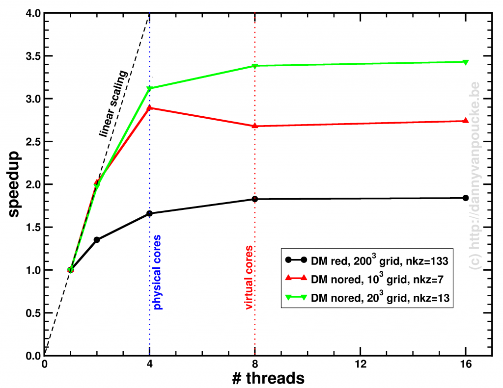
Speedup of the entire phonon-subroutine due to parallelization of the main-phonon-DOS loop.

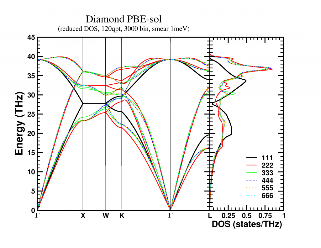
The above graph shows the speed-up results for the two different modes for calculating the phonon-DOS. The reduced mode (DM red), uses a spectrum reduced to that of a unit-cell, but needs a much denser sampling of the Brillouin zone (second approach), and is shown by the black line. The serial calculation in this specific case only took 96 seconds, and the maximum speedup obtained was about x1.84. The red and green curves give the speedup of the calculation mode which makes use of the super-cell spectrum (DM nored, i.e. much larger matrix to solve), and shows for increasing grid sizes a maximum speedup of x2.74 (serial time: 45 seconds) and x3.43 (serial time 395 seconds) respectively. The reason none of the setups reaches a speedup of 4 (or more) is twofold:

  1. Amdahl’s law puts an upper limit to the global speedup of a calculation by taking into account that only part of the code is parallelized (e.g. write sections to a single file can not be parallelized.)
  2. There needs to be sufficient blocks of work for all threads (indicated by nkz in the plot)

In case of the DM nored calculations, the parallelized loop clearly takes the biggest part of the calculation-time, while for the DM red calculation, also the section generating the q-point grid takes a large fraction of the calculation time limiting the effect of parallelization. An improvement here would be to also parallelize  the subroutine generating the grid, but that will be for future work. For now, the expensive DM nored calculations show an acceptable speedup.


Folding Phonons

Game-diamondsAbout a year ago, I discussed the possibility of calculating phonons (the collective vibration of atoms) in the entire Brillouin zone for Metal-Organic Frameworks. Now, one year later, I return to this topic, but this time the subject matter is diamond. In contrast to Metal-Organic Frameworks, the unit-cell of diamond is very small (only 2 atoms). Because a phonon spectrum is calculated through the gradients of forces felt by one atom due to all other atoms, it is clear that within one diamond unit-cell these forces will not be converged. As such, a supercell will be needed to make sure the contribution, due to the most distant atoms, to the experienced forces, are negligible.

Using such a supercell has the unfortunate drawback that the dynamical matrix (which is 3N \times 3N, for N atoms) explodes in size, and, more importantly, that the number of eigenvalues, or phonon-frequencies also increases (3N) where we only want to have 6 frequencies ( 3 \times 2 atoms) for diamond. For an M \times M \times M supercell we end up with 24M^3 -6  additional phonon bands which are the result of band-folding. Or put differently,
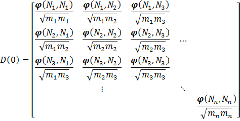
 24M^3 -6 phonon bands coming from the other unit-cells in the supercell. This is not a problem when calculating the phonon density of states. It is, however, a problem when one is interested in the phonon band structure.

The phonon spectrum at a specific q-point in the first Brillouin zone is given by the square root of the eigenvalues of the dynamical matrix of the system. For simplicity, we first assume a finite system of n atoms (a molecule). In that case, the first Brillouin zone is reduced to a single point q=(0,0,0) and the dynamical matrix looks more or less like the hessian:

With \varphi (N_a,N_b) = [\varphi_{i,j}(N_a , N_b)] 3 \times 3 matrices \varphi_{i,j}(N_a,N_b)=\frac{\partial^2\varphi}{\partial x_i(N_a) \partial x_j(N_b)} = - \frac{\partial F_i (N_a)}{\partial x_j (N_b)}  with i, j = x, y, z. Or in words, \varphi_{i,j}(N_a , N_b) represents the derivative of the force felt by atom N_a due to the displacement of atom N_b. Due to Newton’s second law, the dynamical matrix is expected to be symmetric.

When the system under study is no longer a molecule or a finite cluster, but an infinite solid, things get a bit more complicated. For such a solid, we only consider the symmetry in-equivalent atoms (in practice this is often a unit-cell). Because the first Brillouin zone is no longer a single point, one needs to sample multiple different points to get the phonon density-of-states. The role of the q-point is introduced in the dynamical matrix through a factor e^{iq \cdot (r_{N_a} - r_{N_b}) }, creating a dynamical matrix for a single unit-cell containing n atoms:

Because a real solid contains more than a single unit-cell, one should also take into account the interactions of the atoms of one unit-cell with those of all other unit-cells in the system, and as such the dynamical matrix becomes a sum of matrices like the one above:

Where the sum runs over all unit-cells in the system, and Ni indicates an atom in a specific reference unit-cell, and MRi  an atom in the Rth unit-cells, for which we give index 1 to the reference unit-cell. As the forces decay with the distance between the atoms, the infinite sum can be truncated. For a Metal-Organic Framework a unit-cell will quite often suffice. For diamond, however, a larger cell is needed.

An interesting aspect to the dynamical matrix above is that all matrix-elements for a sum over n unit-cells are also present in a single dynamical matrix for a supercell containing these n unit-cells. It becomes even more interesting if one notices that due to translational symmetry one does not need to calculate all elements of the entire supercell dynamical matrix to construct the full supercell dynamical matrix.

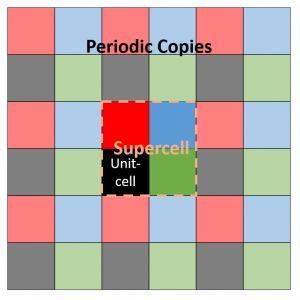
Assume a 2D 2×2 supercell with only a single atom present, which we represent as in the figure on the right. A single periodic copy of the supercell is added in each direction. The dynamical matrix for the supercell can now be constructed as follows: Calculate the elements of the first column (i.e. the gradient of the force felt by the atom in the reference unit-cell, in black, due to the atoms in each of the unit-cells in the supercell). Due to Newton’s third law (action = reaction), this first column and row will have the same elements (middle panel).

Translational symmetry on the other hand will allow us to determine all other elements. The most simple are the diagonal elements, which represent the self-interaction (so all are black squares). The other you can just as easily determine by looking at the schematic representation of the supercell under periodic boundary conditions. For example, to find the derivative of the force on the second cell (=second column, green square in supercell) due to the third cell (third row, blue square in supercell), we look at the square in the same relative position of the blue square to the green square, when starting from the black square: which is the red square (If you read this a couple of times it will start to make sense). Like this, the dynamical matrix of the entire supercell can be constructed.

This final supercell dynamical matrix can, with the same ease, be folded back into the sum of unit-cell dynamical matrices (it becomes an extended lookup-table). The resulting unit-cell dynamical matrix can then be used to create a band structure, which in my case was nicely converged for a 4x4x4 supercell. The bandstructure along high symmetry lines is shown below, but remember that these are actually 3D surfaces. A nice video of the evolution of the first acoustic band (i.e. lowest band) as function of its energy can be found here.

The phonon density of states can also be obtained in two ways, which should, in contrast to the band structure, give the exact same result: (for an M \times M \times M supercell with n atoms per unit-cell)

  1. Generate the density of states for the supercell and corresponding Brillouin zone. This has the advantage that the smaller Brillouin zone can be sampled with fewer q-points, as each q-point acts as M3 q-points in a unit-cell-approach. The drawback here is the fact that for each q-point a (3nM3)x(3nM3) dynamical matrix needs to be solved. This solution scales approximately as O(N3) ~ (3nM3)3 =(3n)3M9. Using linear algebra packages such as LAPACK, this may be done slightly more efficient (but you will not get O(N2) for example).
  2. Generate the density of states for the unit-cell and corresponding Brillouin zone. In this approach, the dynamical matrix to solve is more complex to construct (due to the sum which needs to be taken) but much smaller: 3nx3n. However to get the same q-point density, you will need to calculate M3 times as many q-points as for the supercell.

In the end, the choice will be based on whether you are limited by the accessible memory (when running a 32-bit application, the number of q-point will be detrimental) or CPU-time (solving the dynamical matrix quickly becomes very expensive).


To x64 or not to x64: Installing a 64-bit fortran compiler

Current day computers generally have 64-bit processors, and most even have 64-bit operating systems. On such systems, 32-bit programs will run fine, but 64-bit programs can make more efficient use of the underlying system. When we installed a fortran compiler and the code::blocks IDE, the default fortran compiler generated 32-bit programs. This generally is not an issue, unless you need a large amount of memory, for example to store a temporary array with 4003 double precision coordinates (as I did for a project I’m currently working on). You may first start to look for ways of increasing the stack-size of your program, but you will soon discover that the problem is more profound: a 32-bit program cannot access address spacing beyond 4Gb. (In practice, generally you will not even reach 4Gb before running into problems.) This is because the memory address of your data is stored as a 32-bit value (232 = 4 294 967 296 = 4Gb) so the only way out of this predicament is a “larger address” aka 64-bit. So you need to install a new compiler capable of providing 64-bit programs.

  1. Installing minGW64 for code::blocks
    1. Installing the compiler
    2. Setting the PATH-variable (win10)
    3. Adding the compiler to code::blocks
  2. Upgrading Lapack to 64-bit

Continue reading

One more digit of importance

Over the past few weeks I have bumped into several issues each tracing back to numerical accuracy. Although I have been  programming for almost two decades I never had to worry much about this, making these events seem as-if the universe is trying to tell me something.

Now, let me try to give a proper start to this story; Computational (materials) research is generally perceived as a subset of theoretical (materials) research, and it is true that such a case can be made. It is, however, also true that such thinking can trap us (i.e. the average computational physicist/chemist/mathematician/… programming his/her own code) with numerical accuracy problems. While theoretical equations use exact values for numbers, a computer program is limited by the numerical precision of the variables (e.g. single, double or quadruple precision for real numbers) used in the program. This means that actual numbers with a larger precision are truncated or rounded to the precision of the variable (e.g. 1/3 becomes 0.3333333 instead of 0.333… with an infinite series of 3’s). Most of the time, this is sufficient, and nothing strange will happen. Even more, most of the time, the additional digits would only increase the computational cost while not improving the results in a significant fashion.

Interstellar disc

To understand the importance, or the lack thereof, of additional significant digits, let us first have a look at the precision of \pi and the circumference and surface area of a disc. We will be looking at a rather large disc, one with a radius equal to the distance between the sun, and the nearest star, Alpha Centauri, which is 39 900 000 000 000 km away. The circumference of this disc is given by  2r\pi (or  2.5 \times 10^{14} km ). As a single precision variable \pi will have about 7-8 significant digits. This means the calculated circumference will have an accuracy of about 1 000 000 km (or a few times the distance between the earth and the moon). Using a double precision \pi variable, which has a precision of 16 decimal digits, the circumference will be accurately calculated to within a few meters. At quadrupal precision, the \pi variable would have 34 significant decimal digits, and we would even be able to calculate the surface of the disc ( r^2\pi or  5.0 \times 10^{33} m² ) to within 1 m². Even the surface of a disc the size of our milky way could be calculated with an accuracy of a few hundred square km (or ± the size of Belgium ).

Knowing this, our mind is quickly put at easy regarding possible issues regarding numerical accuracy. However, once in a while we run into one exceptional case (or three, in my case).

1. Infinitesimal finite elements

Temperature profile in the insulating layer of a cylindrical wire.

Temperature profile in the insulating layer of a cylindrical wire.

While looking into the theory behind finite elements, I had some fun implementing a simple program which calculated the temperature distribution due to heat transport in an insulating layer. The finite element approach performed rather nicely, leading to good approximate results, already for a few dozen elements. However, I wanted to push the implementation a bit (the limit of infinite elements should give the exact solution). Since the set of equations was solved by a LAPACK subroutine, using 10 000 elements instead of 10 barely impacted the required time (writing the results took most of 2-3 seconds anyway). The results on the other hand were quite funny as you can see in the picture. The initial implementation, with single precision variables, breaks down even worse already at 1000 elements. Apparently the elements had become too small leading to too small variations of the properties in the stiffness-matrix, resulting in the LAPACK subroutine returning nonsense.

So it turns out that you can have too many elements in a finite elements method.

2. Small volumes: A few more digits please

Optimized volume in Equation of State fit, as function of the range of the fitting data, and step size between data-points. green diamonds, blue triangles and black discs: 1% , 0.5% and 0.25% volume steps respectively.

Optimized volume in Equation of State fit, as function of the range of the fitting data, and step size between data-points. green diamonds, blue triangles and black discs: 1% , 0.5% and 0.25% volume steps respectively.

Recently, I started working at the Wide Band Gap Materials group at the University of Hasselt. So in addition to MOFs I am also working on diamond based materials. While setting up a series of reference calculations, using scripts which already suited me well during my work on MOFs, I was trying to figure out for which volume range, and step size I would get a sufficient convergence in my Equation-of-States Fitting procedure. For the MOFs this is a computationally rather expensive (and tedious) exercise, which, fortunately, gives clear results. For the 2-atom diamond unit cell the calculations are ridiculously fast (in comparison), but the results were confusing. As you can see in the picture, the values I obtained from the different fits seem to oscillate. Checking my E(V) data showed nothing out of the ordinary. All energies and volumes were clearly distinguishable, with the energies given with a precision of 0.001 meV, and the volumes with a precision of 0.01 Å3. However, as you can see in the figure, the volume-oscillations are of the order of 0.001 Å3, ten times smaller than our input precision. Calculating the volumes based on the lattice parameters to get a precision of 10-6 Å3 for the input volumes stabilizes the convergence behavior of the fits (open symbols in the figure). This problem was not present with the MOFs since these have a unit cell volume which is one hundred times larger, so a precision of 0.01 Åmakes the relative error on the volumes one hundred times smaller than was the case for diamond.

In essence, I was trying to get more accurate output than the input I provided, which will never give sensible results (even if they actually look sensible).

3. Many grains of sand really start to pile up after a while

The last one is a bit embarrassing as it lead to a bug in the HIVE-toolbox, which is fixed in the mean time.

One of the HIVE-toolbox users informed me that the dosgrabber routine had crashed because it could not find the Fermi-level in the output of a VASP calculation. Although VASP itself gives a value for the Fermi-level, I do not use it in the above sub-program, since this value tend to be incorrect for spin-polarized systems with different minority and majority spins. However, in an attempt to be smart (and efficient) I ended up in trouble. The basic idea behind my Fermi-level search is just running through the entire Density of States-spectrum until you have counted for all the electrons in the system. Because the VASP estimate for the Fermi-level is not that far of, you do not need to run through the entire list of several thousand entries, but you could just take a subset-centered around the estimated Fermi-level and check in that subset, speeding this up by a factor of 10 to 100. Unfortunately I calculated the energy step size between density of states entries as the difference between the first two entries, which are given to with an accuracy of 0.001 eV. I guess you already have a feeling what will be the problem. When the index of the estimated Fermi-level is 1000, the error will be of the order of 1 eV, which is much larger than the range I took into account. Fortunately, the problem is easily solved by calculating the energy step size as the difference between the first and last index, and divide by the number of steps, making the error in the particular case more than a thousand times smaller.

So, trying to be smart, you always need to make sure you really are being smart, and remember that small number can become very big when there are a lot of them. 

HIVE-STM: A simple post-processing tool for simulating STM

While I was working on my PhD-thesis on Pt nanowires at the university of Twente, one of the things I needed was a method for simulating scanning-tunneling microscopy (STM) images in a quick and easy way. This was because the main experimental information on on these nanowires was contained in STM-images.

Because I love programming, I ended up writing a Delphi-program for this task. Delphi, being an Object Oriented version of the Pascal-programming language containing a Visual Components Library, was ideally suited for writing an easy to use program with a graphical user interface (GUI). The resulting STM-program was specifically designed for my personal needs and the system I was working on at that time.

In August 2008, I was contacted by two German PhD students, with the request if it would be possible for them to use my STM program. In October, an American post-doc and a South-Korean graduate student followed with similar requests, from which point onward I started getting more and more requests from researchers from all over the world. Now, seven years later, I decided to put all “HIVE-users” in a small data-base just to keep track of their number and their affiliation. I already knew I send the program to quite a lot of people, but I was still amazed to discover that it were 225 people from 34 countries.

Hive Requests December 2015

Bar-graph showing the evolution in requests for the HIVE-STM program.

There is a slow but steady increase in requests over the years, with currently on average about one request every week. It is also funny to see there was a slight setback in requests both times I started in a new research-group. For 2015, the data is incomplete, as it does not include all requests of the month December. Another way to distribute the requests is by the month of the year. This is a very interesting graph, since it clearly shows the start of the academic year (October). There are two clear minima (March and September), for which the later is probably related due to the fact that it is the last month of before the start of the academic year (much preparation for new courses) and, in case of the solid state community, this month is also filled with conferences. The reason why there is a minimum in March, however, escapes me ( 💡 all suggestions are welcome 💡 ).

Hive requests per month.

Distribution of requests for the HIVE-STM program on a monthly basis.

The geographic distribution of affiliations of those requesting the STM-program shows Europe, Azia and America to take roughly equal shares, while African affiliations are missing entirety. Hopefully this will change after the workshop on visualization and analysis of VASP outputs delivered at the Center for High Performance Computing‘s 9th National Meeting in South Africa by Dr. David Carballal. By far the most requests come from the USA (57), followed by China(23) and then Germany(15). South-Korea(14) unexpectedly takes the fourth place, while the fifth place is a tie between the UK, Spain and India(12 each).

Hive requests demographics 2015

Distribution of Hive requests per country and continent.

All in all, the STM program seems to be of interest to many more researchers than I would have ever expected, and has currently been cited about 25 times, so it is time to add a page listing these papers as examples of what can be done with HIVE(which has in the mean time been done, check out useful link n°2).

Happy Hiving to all of you, and thank you for your trust.


Useful link:
[1] More information on the HIVE-STM program and how to acquire it.

[2] List of publications using and citing the HIVE-STM program.

Fortran dll’s and libraries: a Progress bar

In the previous fortran tutorials, we learned the initial aspects of object oriented programming (OOP) in fortran 2003. And even though our agent-based opinion-dynamics-code is rather simple, it can quickly take several minutes for a single run of the program to finish. Two tools which quickly become of interest for codes that need more than a few minutes to run are: (1) a progress bar, to track the advance of the “slow” part of the code and prevent you from killing the program 5 seconds before it is to finish, and (2) a timer, allowing you to calculate the time needed to complete certain sections of code, and possibly make predictions of the expected total time of execution.

In this tutorial, we will focus on the progress bar. Since our (hypothetical) code is intended to run on High-Performance Computing (HPC) systems and is written in the fortran language, there generally is no (or no easy) access to GUI’s. So we need our progress bar class to run in a command line user interface. Furthermore, because it is such a widely useful tool we want to build it into a (shared) library (or dll in windows).progress_1pct

The progress bar class

What do we want out of our progress bar? It needs to be easy to use, flexible and smart enough to work nicely even for a lazy user. The output it should provide is formatted as follows: <string> <% progress> <text progress bar>, where the string is a custom character string provided by the user, while ‘%progress’ and ‘text progress bar’ both show the progress. The first shows the progress as an updating number (fine grained), while the second shows it visually as a growing bar (coarse grained).

  1. type, public :: TProgressBar
  2. private
  3. logical :: init
  4. logical :: running
  5. logical :: done
  6. character(len=255) :: message
  7. character(len=30) :: progressString
  8. character(len=20) :: bar
  9. real :: progress
  10. contains
  11. private
  12. procedure,pass(this),public :: initialize
  13. procedure,pass(this),public :: reset
  14. procedure,pass(this),public :: run
  15. procedure,pass(this),private:: printbar
  16. procedure,pass(this),private:: updateBar
  17. end type TProgressBar

All properties of the class are private (data hiding), and only 3 procedures are available to the user: initialize, run and reset. The procedures, printbar and updatebar are private, because we intend the class to be smart enough to decide if a new print and/or update is required. The reset procedure is intended to reset all properties of the class. Although one might consider to make this procedure private as well, it may be useful to allow the user to reset a progress bar in mid progress.(The same goes for the initialize procedure.)

  1. subroutine run(this,pct,Ix,msg)
  2. class(TProgressBar) :: this
  3. real::pct
  4. integer, intent(in), optional :: Ix
  5. character(len=*),intent(in),optional :: msg
  6.  
  7. if (.not. this%init) call this%initialize(msg)
  8. if (.not. this%done) then
  9. this%running=.true.
  10. this%progress=pct
  11. call this%updateBar(Ix)
  12. call this%printbar()
  13. if (abs(pct-100.0)<1.0E-6) then
  14. this%done=.true.
  15. write(*,'(A6)') "] done"
  16. end if
  17. end if
  18.  
  19. end subroutine run

In practice, the run procedure is the heart of the class, and the only procedure needed in most applications. It takes 3 parameters: The progress (pct), the number of digits to print of pct (Ix),and the <string> message (msg). The later two parameters are even optional, since msg may already have been provided if the initialize procedure was called by the user. If the class was not yet initialized it will be done at the start of the procedure. And while the progress bar has not yet reached 100% (within 1 millionth of a %) updates and prints of the bar are performed. Using a set of Boolean properties (init, running, done), the class keeps track of its status. The update and print procedures just do this: update the progress bar data and print the progress bar. To print the progress bar time and time again on the same line, we need to make use of the carriage return character (character 13 of the ASCII table):

write(*,trim(fm), advance='NO') achar(13), trim(this%message),trim(adjustl(this%progressString)),'%','[',trim(adjustl(this%bar))

The advance=’NO‘ option prevents the write statement to move to the next line. This can sometimes have the unwanted side-effect that the write statement above does not appear on the screen. To force this, we can use the fortran 2003 statement flush(OUTPUT_UNIT), where “OUTPUT_UNIT” is a constant defined in the intrinsic fortran 2003 module iso_fortran_env. For older versions of fortran, several compilers provided a (non standard) flush subroutine that could be called to perform the same action. As such, we now have our class ready to be used. The only thing left to do is to turn it into a dll or shared library.progress_25pct

How to create a library and use it

There are two types of libraries: static and dynamic.

Static libraries are used to provide access to functions/subroutines at compile time to the library user. These functions/subroutines are then included in the executable that is being build. In linux environments these will have the extension “.a”, with the .a referring to archive. In a windows environment the extension is “.lib”, for library.

Dynamic libraries are used to provide access to functions/subroutines at run time. In contrast to static libraries, the functions are not included in the executable, making it smaller in size. In linux environments these will have the extension “.so”, with the .so referring to shared object. In a windows environment the extension is “.dll”, for dynamically linked library.

In contrast to C/C++, there is relatively little information to be found on the implementation and use of libraries in fortran. This may be the reason why many available fortran-“libraries” are not really libraries, in the sense meant here. Instead they are just one or more files of fortran code shared by their author(s), and there is nothing wrong with that. These files can then be compiled and used as any other module file.

So how do we create a library from our Progressbar class? Standard examples start from a set of procedures one wants to put in a library. These procedures are put into a .f or .f90 file. Although they are not put into a module (probably due to the idea of having compatibility with fortran 77) which is required for our class, this is not really an issue. The same goes for the .f03 or .f2003 extension for our file containing a fortran 2003 class. To have access to our class and its procedures in our test program, we just need to add the use progressbarsmodule clause. This is because our procedures and class are incorporated in a module (in contrast to the standard examples). Some of the examples I found online also include compiler dependent pragmas to export and import procedures from a dll. Since I am using gfortran+CB for development, and ifort for creating production code, I prefer to avoid such approaches since it hampers workflow and introduces another possible source of bugs.

The compiler setups I present below should not be considered perfect, exhaustive or fool-proof, they are just the ones that work fine for me. I am, however, always very interested in hearing other approaches and fixes in the comments.progress_52pct

Windows

The windows approach is very easy. We let Code::Blocks do all the hard work.

shared library: PBar.dll

Creating the dll : Start a new project, and select the option “Fortran DLL“. Follow the instructions, which are similar to the setup of a standard fortran executable. Modify/replace/add the fortran source you wish to include into your library and build your code (you can not run it since it is a library).

Creating a user program : The program in which you will be using the dll is setup in the usual way. And to get the compilation running smoothly the following steps are required:

  • Add the use myspecificdllmodule clause where needed, with myspecificdllmodule the name of the module included in the dll you wish to use at that specific point.
  • If there are modules included in the dll, the *.mod files need to be present for the compiler to access upon compilation of the user program. (Which results in a limitation with regard to distribution of the dll.)
  • Add the library to the linker settings of the program (project>build options>linker settings), and then add the .dll file.
  • Upon running the program you only need the program executable and the dll.

static library

The entire setup is the same as for the shared library. This time, however, choose the “Fortran Library” option instead of Fortran dll. As the static library is included in the executable, there is no need to ship it with the executable, as is the case for the dll.

Unix

For the unix approach we will be working on the command line, using the intel compiler, since this compiler is often installed at HPC infrastructures.

static library: PBar.a

After having created the appropriate fortran files you wish to include in your library (in our example this is always a single file: PBar.f03, but for multiple files you just need to replace PBar.f03 with the list of files of interest.)

  1. Create the object files:
    ifort -fpic -c -free -Tf Pbar.f03

    Where -fpic tells the compiler to generate position independent code, typical for use in a shared object/library, while -c tells the compiler to create an object file. The -free and -Tf compiler options are there to convince the compiler that the f03 file is actual fortran code to compile and that it is free format.

  2. Use the GNU ar tool to combine the object files into a library:
    ar rc PBarlib.a PBar.o
  3. Compile the program with the library
    ifort TestProgram.f90 PBarlib.a -o TestProgram.exe

    Note that also here the .mod file of our Progressbarsmodule needs to be present for the compilation to be successful.

shared library: PBar.so

For the shared library the approach does not differ that much.

  1. Create the object files:
    ifort -fpic -c -free -Tf Pbar.f03

    In this case the fpic option is not optional in contrast to the static library above. The other options are the same as above.

  2. Compile the object files into a shared library:
    ifort -shared PBar.o -o libPBar.so

    The compiler option -shared creates a shared library, while the -o option allows us to set the name of the library.

  3. Compile the program with the library
    ifort TestProgram.f90 libPBar.so -o TestProgram.exe

    Note that also here the .mod file of our Progressbarsmodule needs to be present for the compilation to be successful. To run the program you also need to add the location of the library file libPBar.so to the environment variable LD_LIBRARY_PATH

One small pickle

HPC systems may perform extensive buffering of data before output, to increase the efficiency of the machine (disk-writes are the slowest memory access option)…and as a result this can sometimes overrule our flush command. The progressbar in turn will not show much progress until it is actually finished, at which point the entire bar will be shown at once. There are options to force the infrastructure not to use this buffering (and the system administrators in general will not appreciate this), for example by setting the compiler flag -assume nobuffered_stdout. So the best solution for HPC applications will be the construction of a slightly modified progress bar, where the carriage return is not used.

progress_100pct


Special thanks also to the people of stack-exchange for clarifying some of the issues with the modules.

Source files for the class and test-program can be downloaded here.