Most commented posts
- Phonons: shake those atoms — 3 comments
- Start to Fortran — 1 comment


Apr 17 2015
Today was the fifth and last day of our spring school on computational tools for materials science. However, this was no reason to sit back and relax. After having been introduced into VASP (day-2) and ABINIT (day-3) for solids, and into Gaussian (day-4) for molecules, today’s code (CP2K) is one which allows you to study both when focusing on dynamics and solvation.
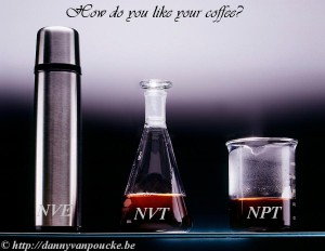
If ensembles were coffee…
The introduction into the Swiss army knife called CP2K was provided by Dr. Andy Van Yperen-De Deyne. He explained to us the nature of the CP2K code (periodic, tools for solvated molecules, and focus on large/huge systems) and its limitations. In contrast to the codes of the previous days, CP2K uses a double basis set: plane waves where the properties are easiest and most accurate described with plane waves and gaussians where it is the case for gaussians. By means of some typical topics of calculations, Andy explained the basic setup of the input and output files, and warned for the explosive nature of too long time steps in molecular dynamics simulations. The possible ensembles for molecular dynamics (MD) were explained as different ways to store hot coffee. Following our daily routine, this session was followed by a hands-on session.
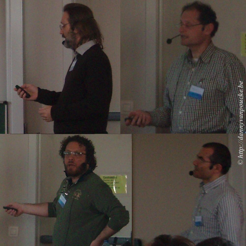
In the afternoon, the advanced session was presented by a triumvirate: Thierry De Meyer, who discussed QM/MM simulations in detail, Dr. Andy Van Yperen-De Deyne, who discused vibrational finger printing and Lennart Joos, who, as the last presenter of the week, showed how different codes can be combined within a single project, each used where they are at the top of their strength, allowing him to unchain his zeolites.

CP2K, all lecturers: Andy Van Yperen-De Deyne (top left), Thierry De Meyer (top right), Lennart Joos (bottom left). All spring school participants hard at work during the hands-on session, even at this last day (bottom right).
The spring school ended with a final hands-on session on CP2K, where the CMM team was present for the last stretch, answering questions and giving final pointers on how to perform simulations, and discussing which code to be most appropriate for each project. At 17h, after my closing remarks, the curtain fell over this spring school on computational tools for materials science. It has been a busy week, and Kurt and I are grateful for the help we got from everyone involved in this spring school, both local and external guests. Tired but happy I look back…and also a little bit forward, hoping and already partially planning a next edition…maybe in two years we will return.
Our external lecturers from the VASP group (Martijn Marsman, top left) and the ABINIT group (Xavier Gonze, top right, Matteo Giantomassi, bottom left, Gian-Marco Rignanese, bottom right)
Apr 16 2015
After having focused on solids during the previous two days of our spring school, using either VASP (Tuesday) or ABINIT (Wednesday), today’s focus goes to molecules, and we turn our attention to the Gaussian code.
Dietmar Hertsen introduced us into the Gaussian code, and immediately showed us why this code was included in our spring school set: it is the most popular code (according to google). He also explained this code is so popular (among chemists) because it can do a lot of the chemistry chemists are interested in, and because of the simplicity of the input files for small molecules. After pointing out the empty lines quirks of Gaussian it was time to introduce some of the possible editors to use with Gaussian. The remainder of his lecture, Dietmar showed us how simple (typical) Gaussian calculations are run, pointing out interesting aspects of the workflow, and the fun of watching vibrations in molden. He ended his lecture giving us some tips and tricks for the investigation of transition states, and the study of chemical reactions, as a mental preparation for the first hands-on session which followed after the coffee-break.
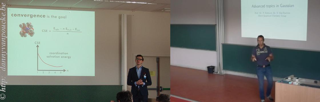
Lecturers for the Gaussian code: Dietmar Hertsen (left) introducing the basics of the code, while Patrick Bultinck (right) discuses more advanced wave function techniques in more detail.
In the afternoon it was time to take out the big guns. Prof. Patrick Bultinck, of the Ghent Quantum Chemistry Group, was so kind to provide the advanced session. In this session, we were reminded, after two days of using the density as a central property, that wave functions are the only way to obtain perfect results. Unfortunately, practical limitations hamper the application to the systems of interest from a practical physical point of view. Patrick, being a quantum chemist to the bone, at several points stepped away from his slides and showed on the blackboard how several approximations to full configuration interaction (full-CI) can be obtained. He also made us aware of the caveats of such approaches; Such as size consistency and basis(-type) dependence for truncated CI, and noted that although CASSCF is a powerful method (albeit not for the fainthearted), it is somewhat a black art that should be used with caution. As such, CASSCF was not included in the advanced hands-on sessions guided by Dr. Sofie Van Damme (but who knows what may happen in a future edition of this spring school).
Apr 15 2015
Today is the third day of our spring school. After the introduction to VASP yesterday, we now turn our attention to another quantum mechanical level solid state code: ABINIT. This is a Belgian ab initio code (mainly) developed at the Université Catholique de Louvain (UCL) in Wallonia.
Since no-one at CMM has practical experience with this code and several of us are interested to learn more about this code, we were very pleased that the group of Prof. Xavier Gonze was willing to support this day in its entirety. During the morning introductory session Prof. Xavier Gonze introduced us into the world of the ABINIT code, for which the initial ideas stem from 1997. Since then, the program has grown to about 800.000 lines of fortran code(!) and a team of 50 people worldwide currently contribute to its development. Also in recent years, a set of python scripts have been developed providing a more user friendly interface (abipy) toward the users of the code. The main goal of the development of this interface, is to shift interest back to the physics instead of trying to figure out which keywords do the trick. We also learned that the ABINIT code is strongly inspired by the ‘free software’ model, and as such Prof. Xavier Gonze prefers to refer to the copyright of ABINIT as copyleft. This open source mentality seems also to provide strength to the code; leading to its large number of developers/contributors; which in turn leads to the implementation of a wide variety of basis-sets, functionals and methodologies.
After the general introduction, Dr. Matteo Giantomassi introduced the abipy python package. This package was especially developed for automating post-processing of ABINIT results, and automatically generating input files. In short, to make interaction with ABINIT easier. Matteo, however, also warned that this approach which makes the use of ABINIT much more black box, might confuse beginners, since a lot of magic is going on under the hood of the abipy scripts. However, his presence, and that of the rest of the ABINIT delegation made sure confusion was kept to a minimum during the hands-on sessions, for which we are very grateful.
After the lunch break, Prof. Gian-Marco Rignanese and Prof. Xavier Gonze held a duo seminar on more advanced topics covering Density Functional Perturbation Theory and based on this spectroscopy and phonon calculations beyond the frozen phonon approach. Of these last aspects I really am interested in seeing how they cope with my Metal Organic Frameworks…
Apr 15 2015
On this second day of our spring school, the first ab initio solid state code is introduced: VASP, the Vienna Ab initio Simulation Package.
Having worked with this code for almost a full decade, some consider me an expert, and as such I had the dubious task of providing first contact with this code to our participants. Since all basic aspects and methods had already been introduced on the first day, I mainly focused on presenting the required input files and parameters, and showing how these should be tweaked for some standard type solid state calculations. Following this one-hour introduction, in which I apparently had not yet scared our participants too much, all participants turned up for the first hands-on session, where they got to play with the VASP program.
In the afternoon, we were delighted to welcome our first invited speaker, straight from the VASP-headquarters: Dr. Martijn Marsman. He introduced us to advanced features of VASP going beyond standard DFT. He showed the power (and limitations) of hybrid-functionals and introduced the quasi-particle approach of GW. We even went beyond GW with the Bethe-Salpeter equations (which include electron-hole interactions). Unfortunately, these much more accurate approaches are also much more expensive than standard DFT, but there is work being done on the implementation of a cubic scaling RPA implementation, which will provide a major step forward in the field of solid state science. Following this session, a second hands-on session took place where exercises linked to these more advanced topic were provided and eagerly tried by many of the more advanced participants.
Apr 13 2015
Today our one-week spring school on computational tools for materials science kicked off. During this week, Kurt Lejaeghere and I host this spring school, which we have been busily organizing the last few months, intended to introduce materials scientists into the use of four major ab-initio codes (VASP, ABINIT, Gaussian and CP2K). During this first day, all participants are immersed in the theoretical background of molecular modeling and solid state physics.

Prof. Karen Hemelsoet presented a general introduction into molecular modeling, showing us which computational techniques are useful to treat problems of varying scales, both in space and time. With the focus going to the modeling of molecules she told us everything there is to know about the potential energy surface, (PES) how to investigate it using different computational methods. She discussed the differences between localized (i.e. gaussian) and plane wave basis sets and taught us how to accurately sample the PES using both molecular dynamics and normal mode analysis. As a final topic she introduced us to the world of computational spectroscopy, showing how infrared spectra can be simulated, and the limitations of this type of simulations.
With the, somewhat mysterious, presentations of Prof. Stefaan Cottenier we moved from the realm of molecules to that of solids. In his first session, he introduced density functional theory, a method ideally suited to treat extended systems at the quantum mechanical level. And showed that as much information is present in the electron density of a system as is in its wave function. In his second session, we fully plunged in the world of solids, and we were guided, step by step, towards a full understanding of the technical details generally found in the methods section of (ab-initio) computational materials science work. Throughout this session, NaCl was used as an ever present example, and we learned that our simple high-school picture of bonding in kitchen salt is a lie-to-children. In reality, Cl doesn’t gain an extra electron by stealing it away from Na, instead it is rather the Na 3s electron which is living to far away from the Na nucleus it belongs to.
Mar 19 2015
It could be that I’ve perhaps found out a little bit about the structure
of atoms. You must not tell anyone anything about it. . .
–Niels Bohr (1885 – 1965),
in a letter to his brother (1912)
Getting the news that a paper got accepted for publication is exciting news, but it can also be a little bit sad since it indicates the end of a project. Little over a month ago we got this great news regarding our paper for the journal of chemical information and modeling. It was the culmination of a side project Goedele Roos and I had been working on, in an on-and-off fashion, over the last two years.
When we started the project each of us had his/her own goal in mind. In my case, it was my interest in showing that my Hirshfeld-I code could handle systems which are huge from the quantum mechanical calculation point of view. Goedele, on the other hand, was interested to see how good Hirshfeld-I charges behaved with increasing size of a molecular fraction. This is of interest for multiscale modeling approaches, for which Martin Karplus, Michael Levitt, and Arieh Warshel got the Nobel prize in chemistry in 2013. In such an approach, a large system, for example a solvated biomolecule containing tens of thousands of atoms, is split into several regions. The smallest central region, containing the part of the molecule one is interested in is studied quantum mechanically, and generally contains a few dozen up to a few hundred atoms. The second shell is much larger, and is described by force-field approaches (i.e. Newtonian mechanics) and can contain ten of thousands of atoms. Even further from the quantum mechanically treated core a third region is described by continuum models.
What about the behavior of the charges? In a quantum mechanical approach, even though we still speak of electrons as-if referring to classical objects, we cannot point to a specific point in space to indicate: “There it is”. We only have a probability distribution in space indicating where the electron may be. As such, it also becomes hard to pinpoint an atom, and in an absolute sense measure/calculate it’s charge. However, because such concepts are so much more intuitive, many chemists and physicists have developed methods, with varying success, to split the electron probability distribution into atoms again. When applying such a scheme on the probability distributions of fractions of a large biomolecule, we would like the atoms at the center not to change to much when the fraction is made larger (i.e. contain more atoms). This would indicate that from some point onward you have included all atoms that interact with the central atoms. I think, you can already see the parallel with the multiscale modeling approach mentioned above; where that point would indicate the boundary between the quantum mechanical and the Newtonian shell.
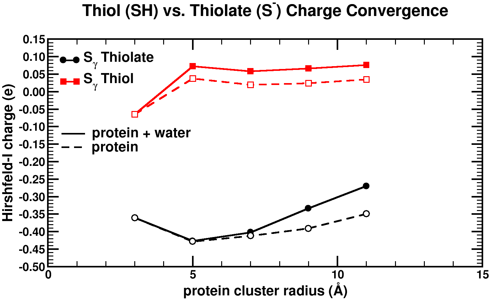
Convergence of Hirshfeld-I charges for clusters of varying size of a biomolecule. The black curves show the charge convergence of an active S atom, while the red curves indicate a deactivated S atom.
Although, we expected to merely be studying this convergence behavior, for the particular partitioning scheme I had implemented, we dug up an unexpected treasure. Of the set of central atoms we were interested all except one showed the nice (and boring) convergence behavior. The exception (a sulfur atom) showed a clear lack of convergence, it didn’t even show any intend toward convergence behavior even for our system containing almost 1000 atoms. However, unlike the other atoms we were checking, this S atom had a special role in the biomolecule: it was an active site, i.e. the atom where chemical reactions of the biomolecule with whatever else of molecule/atom are expected to occur.
Because this S atom had a formal charge of -1, we bound a H atom to it, and investigated this set of new fractions. In this case, the S atom, with the H atom bound to it, was no longer an active site. Lo and behold, the S atom shows perfect convergence like all other atoms of the central cluster. This shows us that an active site is more than an atom sitting at the right place at the right time. It is an atom which is reaching out to the world, interacting with other atoms over a very long range, drawing them in (>10 ångström=1 nm is very far on the atomic scale, imagine it like being able to touch someone who is standing >20 m away from you). Unfortunately, this is rather bad news for multiscale modeling, since this means that if you want to describe such an active site accurately you will need an extremely large central quantum mechanical region. When the active site is deactivated, on the other hand, a radius of ~0.5 nm around the deactivated site is already sufficient.
Similar to Bohr, I have the feeling that “It could be that I’ve perhaps found out a little bit about the structure
of atoms.”, and it makes me happy.
Mar 02 2015
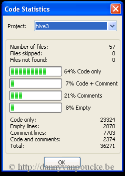
Code-statistics for the hive3 code (feb.2015)
If you are used to programming in C/C++, Java or Pascal, you probably do this using an Integrated Development Environment (IDE’s) such as Dev-Cpp/Pascal, Netbeans, Eclipse, … There are dozens of free IDE’s for each of these languages. When starting to use fortran, you are in for a bit of a surprise. There are some commercial IDE’s that can handle fortran (MS Visual Studio, or the Lahey IDE). Free fortran IDEs are rather scarce and quite often are the result of the extension of a C++ focused IDE. This, however, does not make them less useful. Code::Blocks is such an IDE. It supports several programming and scripting languages including C and fortran, making it also suited for mixed languages development. In addition, this IDE has been developed for Windows, Linux and Mac Os X, making it highly portable. Furthermore, installing this IDE combined with for example the gcc compiler can be done quickly and without much hassle, as is explained in this excellent tutorial. In 5 steps everything is installed and you are up and running:
Go for binaries and get the installer if you are using Windows. This will provide you with the latest build. Be careful if you are doing this while upgrading from gfortran 4.8 to 4.9 or 4.10. The latter two are known to have a recently fixed compiler-bug related to the automatic finalization of objects. A solution to this problem is given in this post.
UPDATE 03/02/2017: As the gcc page has changed significantly since this post was written, I suggest to follow the procedure described here for the installation of a 64bit version of the compiler.
Since version 13.12 the Fortranproject plugin is included in the Code::Blocks installation.
Run the installer obtained at step 1…i.e. keep clicking OK until all is finished.
Of course any real project will contain many files, and when you start to create fortran 2003/2008 code you will want to use “.f2003” or “.f03” instead of “.f90” . The Code::Blocks IDE is well suited for the former tasks, and we will return to these later. Playing with this IDE is the only way to learn about all its options. Two really nice plugins are “Format Fortran Indent” and “Code statistics”. The first one can be used to auto-indent your Fortran code, making it easier to find those nasty missing “end” statements. The code statistics tool runs through your entire project and tells you how many lines of code you have, and how many lines contain comments.
Feb 21 2015
(source via Geographical Perspectives)
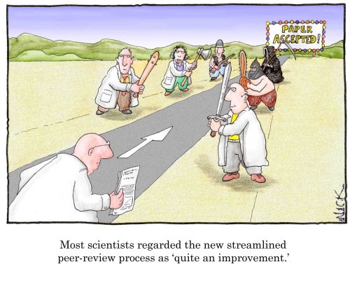
The last three months have been largely dedicated to the review of publications: On the one hand, some of my own work was going through the review-process, while on the other hand, I myself had to review several publications for various journals. During this time I got to see the review reports of fellow reviewers, both for my own work and the work I had to reviewed. Because the peer-review experience is an integral part of modern science, some hints for both authors and reviewers:
When you get your first request to review a paper for a peer reviewed journal‡, this is an exciting experience. It implies you are being recognized by the community as a scientist with some merit. However, as time goes by, you will see the number of these requests increase, and your available time decreases (this is a law of nature). As such, don’t be too eager to press that accept button. If you do not have time to do it this week, chances are slim you will have time next week or the week after that. Only accept when you have time to do it NOW. This ensures that you can provide a qualitative report on the paper under review (cf. point below) No-one will be angry if you say no once in a while. Some journals also ask if you can suggest alternate reviewers in such a case. As a group group leader (or more senior scientist) this is a good opportunity to introduce more junior scientists into the review process.
‡ Not to be mistaken with predatory journals, presenting all kinds of schemes in which you pay heavily for your publication to get published.
You have always been selected specifically for your qualities, which in some cases means your name came up in a google search combining relevant keywords (not only authors and reviewers are victims of the current publish-or-perish mentality). Don’t be afraid to decline if a paper is outside your scope of interest/understanding. In my own case, I quite often get the request to review experimental papers which I will generally decline, unless I the abstract catches my interest. In such a case, it is best to let the editor know via a private note that although you provide a detailed report, you expect there to be an actual specialist (in my case an experimentalist) present with the other reviewers which can judge the specialized experimental aspects of the work you are reviewing.
In some fields it is normal for the review process to be double blind (authors do not know the reviewers, and the reviewers do not know the authors), in others this is not the case. However, to be able to review a paper on it’s merit try to ignore who the authors are, it should reduce bias (both favorable or unfavorable), because that is the idea of science and writing papers: it should be about the work/science not the people who did the science.
Single sentence reviews stating how good/bad a paper is, only shows you barely looked at it (this may be due to time constraints or being outside your scope of expertise: cf. above). Although it may be nice for the authors to hear you found their work great and it should be published immediately, it leaves a bit of a hollow sense. In case of a rejection, on the other hand it will frustrate the authors since they do not learn anything from this report. So how can they ever improve it?
No matter how good paper, one can always make remarks. Going from typographical/grammatical issues (remember, most authors are not native English speakers) to conceptual issues, aspects which may be unclear. Never be afraid to add these to your report.
Although this is a quite a obvious statement, there appear to be authors who just send in their draft to a high ranking journal to get a review-report and then use this to clean up the draft and send it elsewhere. When you submit a paper you should always have the intention of having it accepted and published, and not just use the review progress to point out the holes in your current work in progress.
Some people like to make figures and tables, others don’t. If you are one of the latter, whatever you do, avoid making sloppy figures or tables (e.g. incomplete captions, missing or meaningless legends, label your axis, remove artifacts from your graphics software, or even better switch to other graphics software). Tables and figures are capitalized because they are a neat and easy to use means of transferring information from the author to the reader. In the end it is often better not to have a figure/table than to have a bad one.
Although as a species we are called homo sapiens (wise man) in essence we are rather pan narrans (storytelling chimpanzee). We tell stories, and have always told stories, to transfer knowledge from one generation to another. Fairy-tales learn us a dark forest is a dangerous place while proverbs express a truth based on common sens and practical experience.
As such, a good publication is also more than just a cold enumeration of a set of data. You can order you data to have a story-line. This can be significantly different from the order in which you did your work. You could just imagine how you could have obtained the same results in a perfect world (with 20/20 hindsight that is a lot easier) and present steps which have a logical order in that (imaginary) perfect world. This will make it much easier for your reader to get through the entire paper. Note that it is often easier to have a story-line for a short piece of work than a very long paper. However, in the latter case the story-line is even more important, since it will make it easier for your reader to recollect specific aspects of your work, and easily track them down again without the need to go through the entire paper again.
Some journals allow authors to provide SI to their work. This should be data, to my opinion, without which the paper also can be published. Here you can put figures/tables which present data from the publication in a different format/relation. You can also place similar data in the SI: E.g. you have a dozen samples, and you show a spectrum of one sample as a prototype in the paper, while the spectra of the other samples are placed in SI. What you should not do is put part of the work in the SI to save space in the paper. Also, something I have seen happen is so-called combined experimental-theoretical papers, where the theoretical part is 95% located in the SI, only the conclusions of the theoretical part are put in the paper itself. Neither should you do the reverse. In the end you should ask yourself the question: would this paper be published/publishable under the same standards without the information placed in SI. If the answer is yes, then you have placed the right information in the SI.
Since many, if not all, funding organisations and promotion committees use the number of publications as a first measure of merit of a scientist, this leads to a very unhealthy idea that more publications means better science. Where the big names of 50 years ago could actually manage to have their first publication as a second year post doc, current day researchers (in science and engineering) will generally not even get their PhD without at least a handful publications. The economic notion of ever increasing profits (which is a great idea, as we know since the economic crisis of 2008) unfortunately also transpires in science, where the number of publications is the measure of profit. This sometimes drives scientists to consider publishing “Least Publishable Units”. Although it is true that it is easier to have a story-line for a short piece of work, you also loose the bigger picture. If you consider splitting your work in separate pieces, consider carefully why you do this. Should you do this? Fear that a paper will be too long is a poor excuse, since you can structure your work. Is there actually anything to gain scientifically from this, except one additional publication? Funding agencies claim to want only excellent work; so remind them that excellent work is not measured in simple accounting numbers.
Disclaimer: These hints reflect my personal opinion/preferences and as such might differ from the opinion/preference of your supervisor/colleagues/…, but I hope they can provide you an initial guide in your own relation to the peer-review process.
Feb 10 2015
| Authors: | Danny E. P. Vanpoucke, Julianna Oláh, Frank De Proft, Veronique Van Speybroeck, and Goedele Roos |
| Journal: | J. Chem. Inf. Model. 55(3), 564-571 (2015) |
| doi: | 10.1021/ci5006417 |
| IF(2015): | 3.657 |
| export: | bibtex |
| pdf: | <J.Chem.Inf.Model.> |
 |
| Graphical Abstract: Graphical Abstract: The influence of the cluster size and water presence on the atomic charge of active and inactive sites in Bio-molecules. |
Atomic charges are a key concept to give more insight into the electronic structure and chemical reactivity. The Hirshfeld-I partitioning scheme applied to the model protein human 2-cysteine peroxiredoxin thioredoxin peroxidase B is used to investigate how large a protein fragment needs to be in order to achieve convergence of the atomic charge of both, neutral and negatively charged residues. Convergence in atomic charges is rapidly reached for neutral residues, but not for negatively charged ones. This study pinpoints difficulties on the road towards accurate modeling of negatively charged residues of large bio-molecular systems in a multiscale approach.
Feb 07 2015
Fortran, just like COBOL (not to be confused with cobold), is a programming language which is most widely known for its predicted demise. It has been around for over half a century, making it the oldest high level programming language. Due to this age, it is perceived by many to be a language that should have gone the way of the dinosaur a long time ago, however, it seems to persist, despite futile attempts to retire it. One of the main concerns is that the language is not up to date, and there are so many nice high level languages which allow you to do things much easier and “as fast”. Before we look into that, it is important to know that there are roughly two types of programming languages:
The former languages result in binary code that is executed directly on the machine of the user. These programs are generally speaking fast and efficient. Their drawback, however, is that they are not very transferable (different hardware, e.g. 32 vs. 64 bit, tend to be a problem). In contrast, interpreted languages are ‘compiled/interpreted’ at run-time by additional software installed on the machine of the user (e.g. JVM: Java virtual machine), making these scripts rather slow and inefficient since they are reinterpreted on each run. Their advantage, however, is their transferability and ease of use. Note that Java is a bit of a borderline case; it is not entirely a full programming language like C and Fortran, since it requires a JVM to run, however, it is also not a pure scripting language like python or bash where the language is mainly used to glue other programs together.
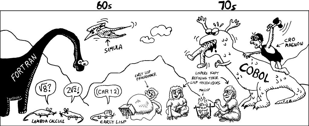
Fortran has been around since the age of the dinosaurs. (via Onionesque Reality)
Now let us return to Fortran. As seen above, it is a compiled language, making it pretty fast. It was designed for scientific number-crunching purposes (FORTRAN comes from FORmula TRANslation) and as such it is used in many numerical high performance libraries (e.g. (sca) LAPACK and BLAS). The fact that it appeared in 1957 does not mean nothing has happened since. Over the years the language evolved from a procedural language, in FORTRAN II, to one supporting also modern Object Oriented Programming (OOP) techniques, in Fortran 2003. It is true that new techniques were introduced later than it was the case in other languages (e.g. the OOP concept), and many existing scientific codes contain quite some “old school” FORTRAN 77. This gives the impression that the language is rather limited compared to a modern language like C++.
So why is it still in use? Due to its age, many (numerical) libraries exist written in Fortran, and due to its performance in a HPC environment. This last point is also a cause of much debate between Fortran and C adepts. Which one is faster? This depends on many things. Over the years compilers have been developed for both languages aiming at speed. In addition to the compiler, also the programming skills of the scientist writing the code are of importance. As a result, comparative tests end up showing very little difference in performance [link1, link2]. In the end, for scientific programming, I think the most important aspect to consider is the fact that most scientist are not that good at programming as they would like/think (author included), and as such, the difference between C(++) and Fortran speeds for new projects will mainly be due to this lack of skills.
However, if you have no previous programming experience, I think Fortran may be easier and safer to learn (you can not play with pointers as is possible with C(++) and Pascal, which is a good thing, and you are required to define your variables, another good coding practice (Okay, you can use implicit typing in theory, but more or less everybody will suggest against this, since it is bad coding practice)). It is also easier to write more or less bug free code than is possible in C(++) (remember defining a global constant PI and ending up with the integer value 3 instead of 3.1415…). Also its long standing procedural setup keeps things a bit more simple, without the need to dive into the nitty gritty details of OOP, where you should know that you are handling pointers (This may be news for people used to Java, and explain some odd unexpected behavior) and getting to grips with concepts like inheritance and polymorphism, which, to my opinion, are rather complex in C++.
In addition, Fortran allows you to grow, while retaining ‘old’ code. You can start out with simple procedural design (Fortran 95) and move toward Object Oriented Programming (Fortran 2003) easily. My own Fortran code is a mixture of Fortran 95 and Fortran 2003. (Note for those who think code written using OOP is much slower than procedural programming: you should set the relevant compiler flags, like –ipo )
In conclusion, we end up with a programming language which is fast, if not the fastest, and contains most modern features (like OOP). Unlike some more recent languages, it has a more limited user base since it is not that extensively used for commercial purposes, leading to a slower development of the compilers (though these are moving along nicely, and probably will still be moving along nicely when most of the new languages have already been forgotten again). Tracking the popularity of programming languages is a nice pastime, which will generally show you C/C++ being one of the most popular languages, while languages like Pascal and Fortran dangle somewhere around 20th-40th position, and remain there over long timescales.
The fact that Fortran is considered rather obscure by proponents of newer scripting languages like Python can lead to slightly funny comment like:“Why don’t you use Python instead of such an old and deprecated language, it is so such easier to use and with the NumPy and SciPy library you can also do number-crunching.”. First of all, Python is a scripting language (which in my mind unfortunately puts it at about the same level as HTML and CSS 🙂 ), but more interestingly, those libraries are merely wrappers around C-wrappers around FORTRAN 77 libraries like MINPACK. So people suggesting to use Python over Fortran 95/2003 code, are actually suggesting using FORTRAN 77 over more recent Fortran standards. Such comments just put a smile on my face. 😀 With all this in mind, I hope to show in this blog that modern Fortran can tackle all challenges of modern scientific programming.