Materials properties, such as the electronic structure, depend on the atomic structure of a material. For this reason it is important to optimize the atomic structure of the material you are investigating. Generally you want your system to be in the global ground state, which, for some systems, can be very hard to find. This can be due to large barriers between different conformers, making it easy to get stuck in a local minimum. However, a very shallow energy surface will be problematic as well, since optimization algorithms can get stuck wandering these plains forever, hopping between different local minima (Metal-Organic Frameworks (MOFs) and other porous materials like Covalent-Organic Frameworks and Zeolites are nice examples).
VASP, as well as other ab initio software, provides multiple settings and possibilities to perform structure optimization. Let’s give a small overview, which I also present in my general VASP introductory tutorial, in order of increasing workload on the user:
- Experimental Structure: This the most lazy option, as it entails just taking an experimentally obtained structure and not optimizing it at all. This should be avoided unless you have a very specific reason why you want to use specifically this geometry. (In this regard, Force-Field optimized structures fall into the same category.)
- Simple VASP Optimization: You can let VASP do the heavy lifting. There are several parameters which help with this task.
- IBRION = 1 (RMM-DIIS, good close to a minimum), 2 (conjugate gradient, safe for difficult problems, should always work), 3 (damped molecular dynamics, useful if you start from a bad initial guess) The IBRION tag determines how ions are moved during relaxation.
- ISIF = 2 (Ions only, fixed shape and volume), 4 (Ions and cell shape, fixed volume), 3 (ions, shape and volume relaxed) The ISIF tag determines how the stress tensor is calculated, and which degrees of freedom can change during a relaxation.
- ENCUT = max(ENMAX)x1.3 To reduce Pulay stresses, it is advised to increase the basis set to 1.3x the default value, which is the largest ENMAX value for the atoms used in your system.
- Volume Scan (Quick and dirty): For many systems, especially simple systems, the internal coordinates of the ions are often well represented in available structure files. The main parameter which needs optimization is the lattice parameter. This is also often the main change if different functional are used. In a quick and dirty volume scan, one performs a set of static calculations, only the volume of the cell is changed. The shape of the cell and the internal atom coordinates are kept fixed. Fitting a polynomial to the resulting Energy-Volume data can then be used to obtain the optimum volume. This option is mainly useful as an initial guess and should either be followed by option 2, or improved to option 4.
- Equation of state fitting to fixed volume optimized structures: This approach is the most accurate (and expensive) method. Because you make use of fixed volume optimizations (ISIF = 4), the errors due to Pulay stresses are removed. They are still present for each separate fixed volume calculation, but the equation of state fit will average out the basis-set incompleteness, as long as you take a large enough volume range: 5-10%. Note that the 5-10% volume range is generally true for small systems. In case of porous materials, like MOFs, ±4% can cover a large volume range of over 100 Å3. Below you can see a pseudo-code algorithm for this setup. Note that the relaxation part is split up in several consecutive relaxations. This is done to further reduce basis-set incompleteness errors. Although the cell volume does not change, the shape does, and the original sphere of G-vectors is transformed into an ellipse. At each restart this is corrected to again give a sphere of G-vectors. For many systems the effect may be very small, but this is not always the case, and it can be recognized as jumps in the energy going from one relaxation calculation to the next. The convergence is set the usual way for a relaxation in VASP (EDIFF and EDIFFG parameters) and a threshold in the number of ionic steps should be set as well (5-10 for normal systems is reasonable, while for porous/flexible materials you may prefer a higher value). There exist several possible equations-of-state which can be used for the fit of the E(V) data. The EOSfit option of HIVE-4 implements 3:
- Birch-Murnaghan third order isothermal equation of state
- Murnaghan equation of state
- Rose-Vinet equation of state (very well suited for (flexible) MOFs)
Using the obtained equilibrium volume a final round of fixed volume relaxations should be done to get the fully optimized structure.
[codesyntax lang=”c” title=”Pseudo-code”]
For (set of Volumes: equilibrium volume ±5%){
	Step 1          : Fixed Volume relaxation
	(IBRION = 2, ISIF=4, ENCUT = 1.3x ENMAX, LCHARG=.TRUE., NSW=100)
	Step 2→n-1: Second and following fixed Volume relaxation (until a threshold is crossed and the structure is relaxed in fewer than N ionic steps) (IBRION = 2, ISIF=4, ENCUT = 1.3x ENMAX, ICHARG=1, LCHARG=.TRUE., NSW=100)
	Step n : Static calculation (IBRION = -1, no ISIF parameter, ICHARG=1, ENCUT = 1.3x ENMAX, ICHARG=1, LCHARG=.TRUE., NSW=0)
}
Fit Volume-Energy to Equation of State.
Fixed volume relaxation at equilibrium volume. (With continuations if too many ionic steps are required.)
Static calculation at equilibrium volume
[/codesyntax]
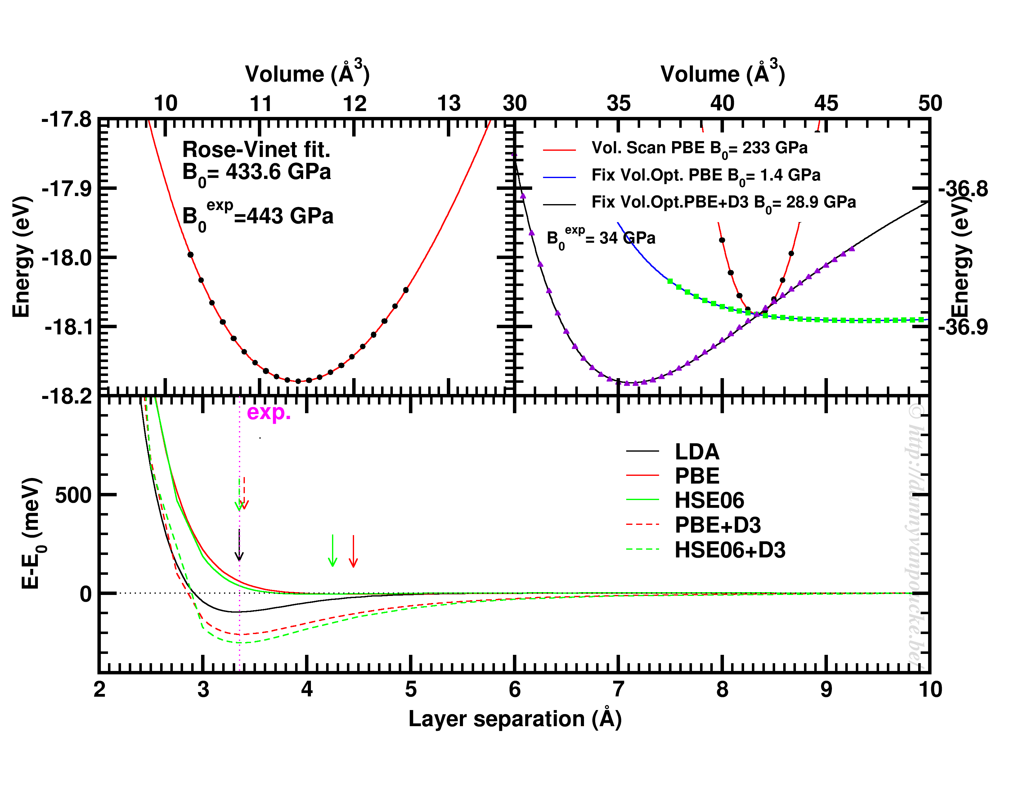
Top-left: Volume scan of Diamond. Top-right: comparison of volume scan and equation of state fitting to fixed volume optimizations, showing the role of van der Waals interactions. Bottom: Inter-layer binding in graphite for different functionals.
Some examples
Let us start with a simple and well behaved system: Diamond. This material has a very simple internal structure. As a result, the internal coordinates should not be expected to change with reasonable volume variations. As such, a simple volume scan (option 3), will allow for a good estimate of the equilibrium volume. The obtained bulk modulus is off by about 2% which is very good.
Switching to graphite, makes things a lot more interesting. A simple volume scan gives an equilibrium volume which is a serious overestimation of the experimental volume (which is about 35 Å3), mainly due to the overestimation of the c-axis. The bulk modulus is calculated to be 233 GPa a factor 7 too large. Allowing the structure to relax at fixed volume changes the picture dramatically. The bulk modulus drops by 2 orders of magnitude (now it is about 24x too small) and the equilibrium volume becomes even larger. We are facing a serious problem for this system. The origin lies in the van der Waals interactions. These weak forces are not included in standard DFT, as a result, the distance between the graphene sheets in graphite is gravely overestimated. Luckily several schemes exist to include these van der Waals forces, the Grimme D3 corrections are one of them. Including these the correct behavior of graphite can be predicted using an equation of state fit to fixed volume optimizations.(Note that the energy curve was shifted upward to make the data-point at 41 Å3 coincide with that of the other calculations.) In this case the equilibrium volume is correctly estimated to be about 35 Å3 and the bulk modulus is 28.9 GPa, a mere 15% off from the experimental one, which is near perfect compared to the standard DFT values we had before.
In case of graphite, the simple volume scan approach can also be used for something else. As this approach is well suited to check the behaviour of 1 single internal parameter, we use it to investigate the inter-layer interaction. Keeping the a and b lattice vectors fixed, the c-lattice vector is scanned. Interestingly the LDA functional, which is known to overbind, finds the experimental lattice spacing, while both PBE and HSE06 overestimate it significantly. Introducing D3 corrections for these functionals fixes the problem, and give a stronger binding than LDA.
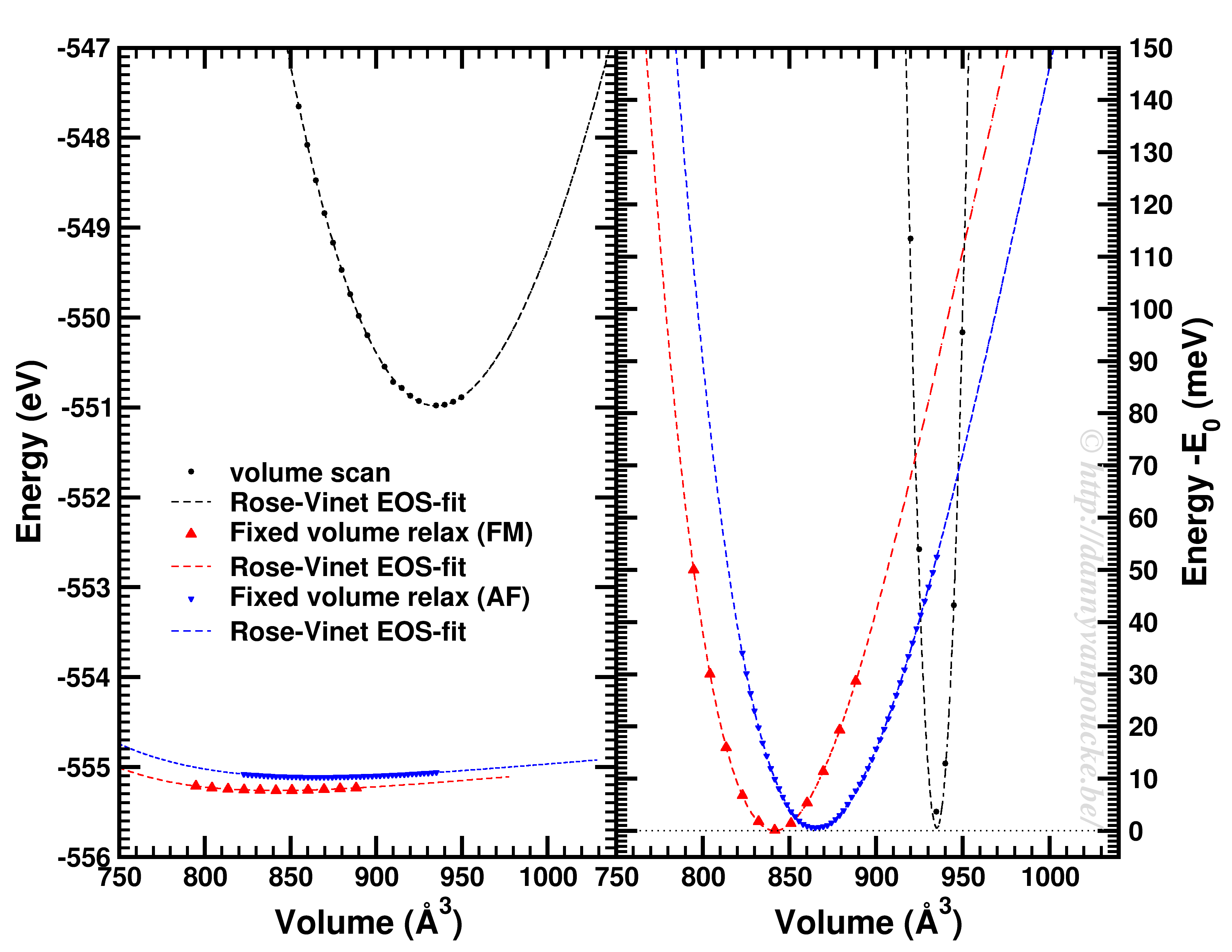
Comparison of a volume scan and an EOS-fit to fixed volume optimizations for a Metal-Organic Framework with MIL53/47 topology.
We just saw that for simple systems, the simple volume scan can already be too simple. For more complex systems like MOFs, similar problems can be seen. The simple volume scan, as for graphite gives a too sharp potential (with a very large bulk modulus). In addition, internal reordering of the atoms gives rise to very large changes in the energy, and the equilibrium volume can move quite a lot. It even depends on the spin-configuration.
In conclusion: the safest way to get a good equilibrium volume is unfortunately also the most expensive way. By means of an equation of state fit to a set of fixed volume structure optimizations the ground state (experimental) equilibrium volume can be found. As a bonus, the bulk modulus is obtained as well.


 Today is a joyful day, as I am getting married to my lovely girlfriend, my partner in crime, the mother of our son, the stars of my night-sky: my wife.


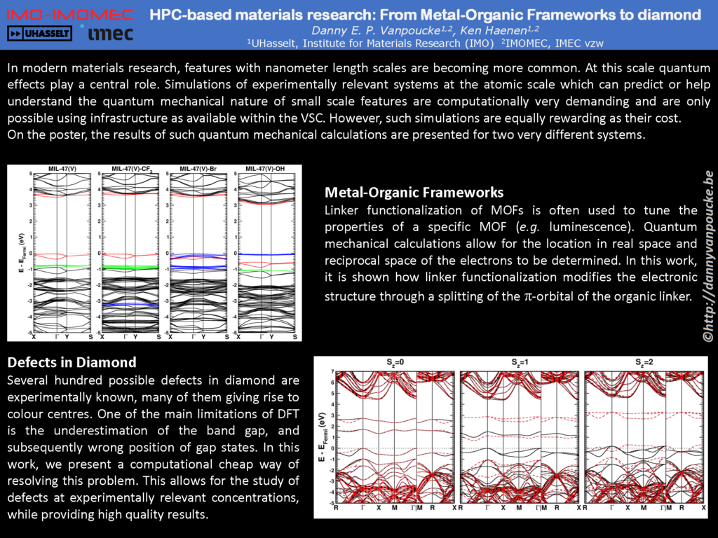
 upon OH-functionalization of the BDC linker.")