Most commented posts
- Start to Fortran — 1 comment
- Phonons: shake those atoms — 3 comments


Mar 08 2017
For a recent project, attempting to investigate Eu dopants in bulk diamond, I ended up simplifying the problem and investigating the C-vacancy in diamond. The setup is simple: take a super cell of diamond, remove 1 carbon atom and calculate. This, however, ended up being a bit more complicated than I had expected.
Removing the single carbon atom gives rise to 4 dangling bonds on the neighboring carbon atoms. The electrons occupying these bonds will gladly interact with one another, giving rise to three different possible spin states:
Starting the calculations without any assumptions gives nice results. Unfortunately they are wrong, and we seem to have ended up in nearby local minima. Including the spin-configurations above as starting assumptions solves the problem, luckily.
The electronic structure is, however, still not a perfect match for experiment. But this is well-known behavior for Density Functional Theory with local functionals such as LDA and PBE. A solution is the use of hybrid functionals (such as HSE06). Conservation of misery kicks in hard at this point, since the latter type of calculations are 1000x as expensive in compute time (and the LDA and PBE calculations aren’t finished in a matter of seconds or minutes, but need several hours on multiple cores). An old methodology to circumvent this problem is the use of Hubbard-U like correction terms (so-called DFT+U). Interestingly for this defect system the two available parameters in a DFT+U setup are independent, and allow for the electronic structure to be perfectly tuned. At the end of the fitting exercise, we now have two additional parameters, which allow us to get electronic structures of hybrid functional quality, but at PBE computational cost.
The evolution of the band-structure as function of the two parameters can be seen below.
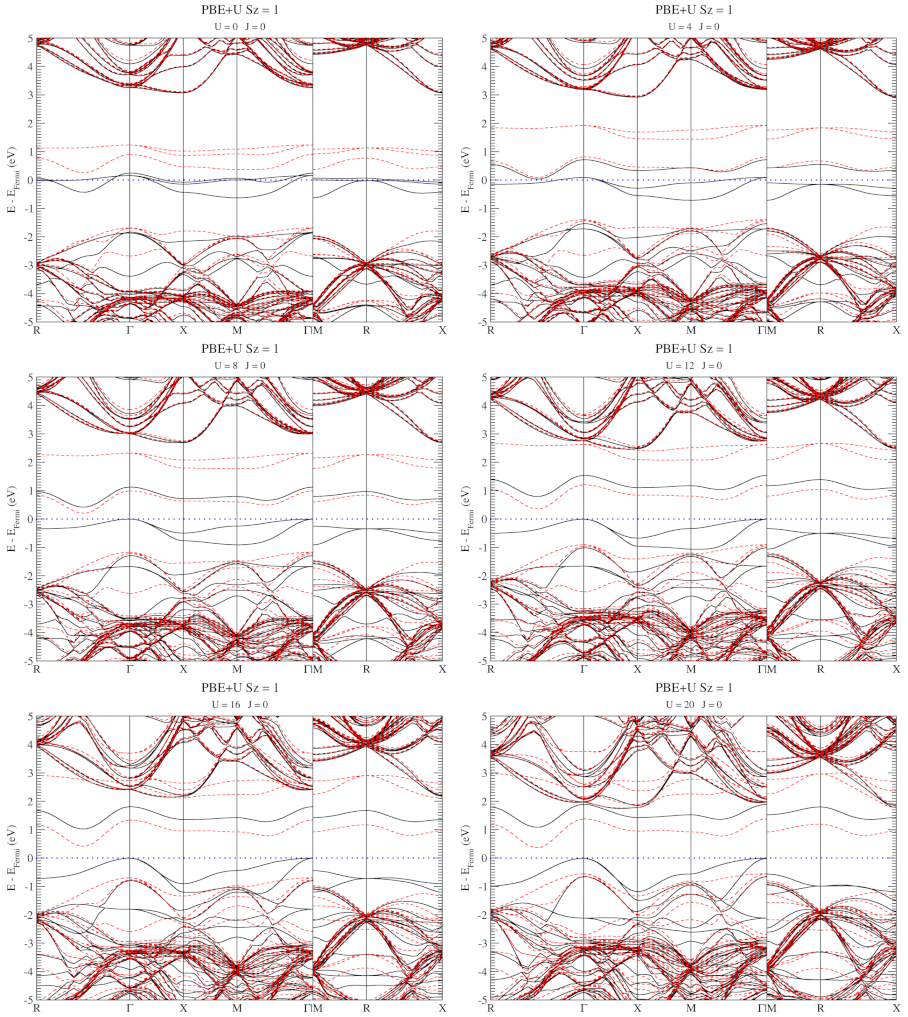
DFT+U series (varying U) for a specific spin state of the C-vacancy defect.
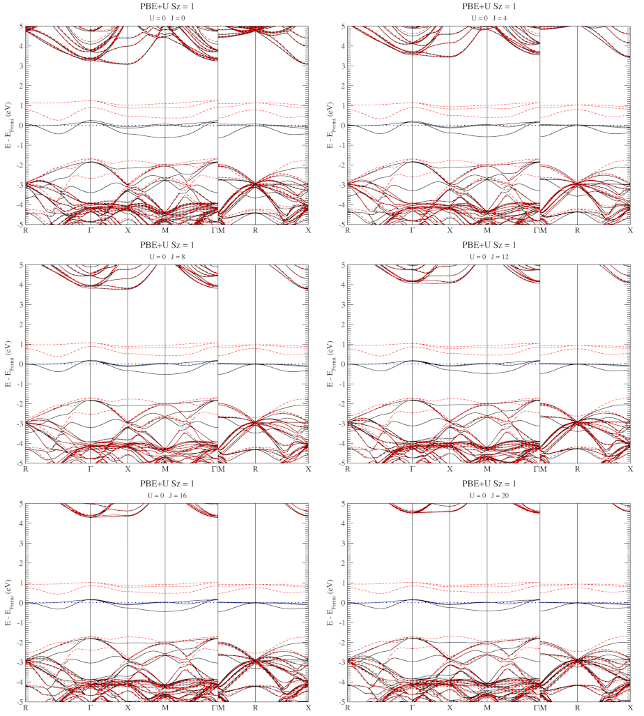
DFT+U series (varying J) for a specific spin state of the C-vacancy defect.
Permanent link to this article: https://dannyvanpoucke.be/diamond-dftu-en/
Jan 06 2017
Materials properties, such as the electronic structure, depend on the atomic structure of a material. For this reason it is important to optimize the atomic structure of the material you are investigating. Generally you want your system to be in the global ground state, which, for some systems, can be very hard to find. This can be due to large barriers between different conformers, making it easy to get stuck in a local minimum. However, a very shallow energy surface will be problematic as well, since optimization algorithms can get stuck wandering these plains forever, hopping between different local minima (Metal-Organic Frameworks (MOFs) and other porous materials like Covalent-Organic Frameworks and Zeolites are nice examples).
VASP, as well as other ab initio software, provides multiple settings and possibilities to perform structure optimization. Let’s give a small overview, which I also present in my general VASP introductory tutorial, in order of increasing workload on the user:
Using the obtained equilibrium volume a final round of fixed volume relaxations should be done to get the fully optimized structure.
[codesyntax lang=”c” title=”Pseudo-code”]
For (set of Volumes: equilibrium volume ±5%){
	Step 1          : Fixed Volume relaxation
	(IBRION = 2, ISIF=4, ENCUT = 1.3x ENMAX, LCHARG=.TRUE., NSW=100)
	Step 2→n-1: Second and following fixed Volume relaxation (until a threshold is crossed and the structure is relaxed in fewer than N ionic steps) (IBRION = 2, ISIF=4, ENCUT = 1.3x ENMAX, ICHARG=1, LCHARG=.TRUE., NSW=100)
	Step n : Static calculation (IBRION = -1, no ISIF parameter, ICHARG=1, ENCUT = 1.3x ENMAX, ICHARG=1, LCHARG=.TRUE., NSW=0)
}
Fit Volume-Energy to Equation of State.
Fixed volume relaxation at equilibrium volume. (With continuations if too many ionic steps are required.)
Static calculation at equilibrium volume
[/codesyntax]
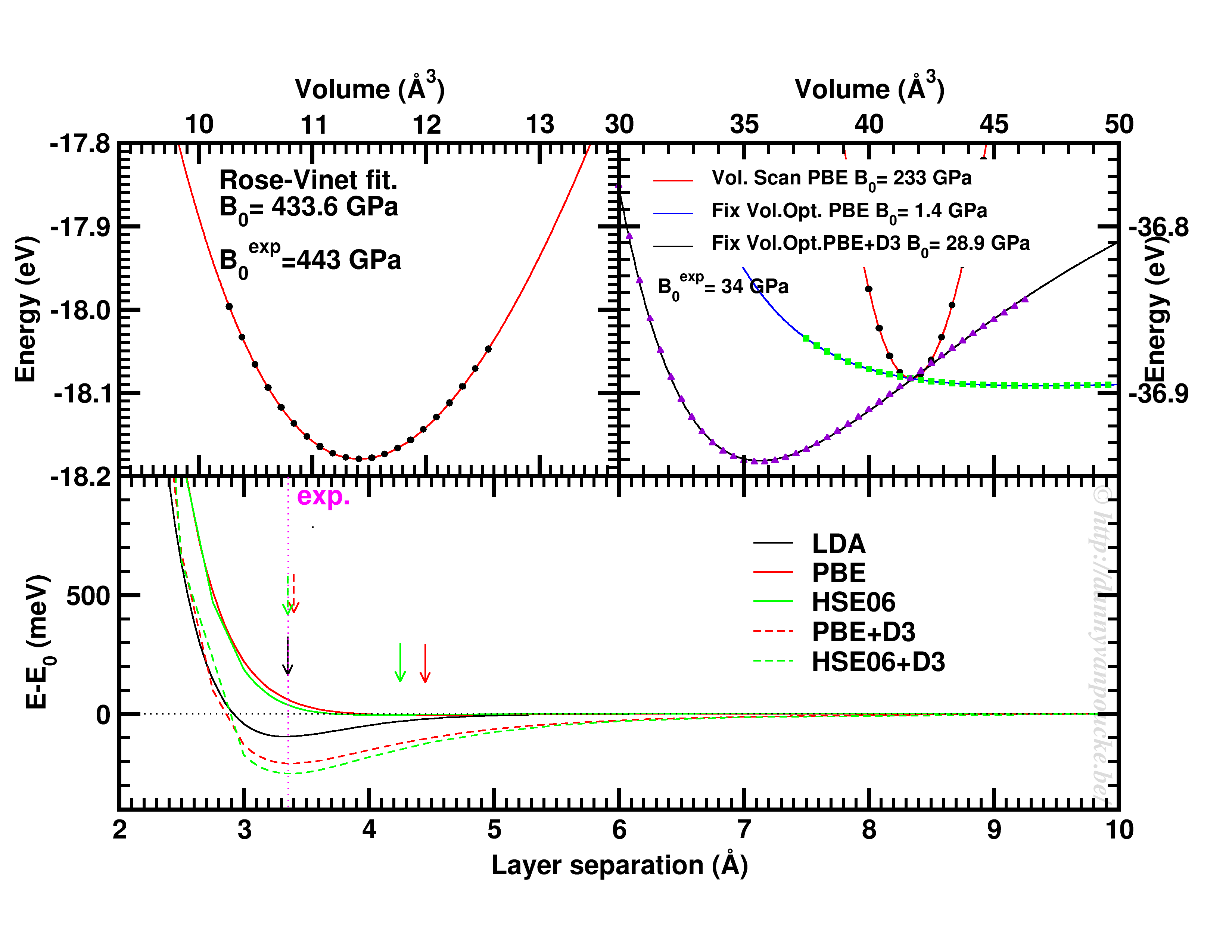
Top-left: Volume scan of Diamond. Top-right: comparison of volume scan and equation of state fitting to fixed volume optimizations, showing the role of van der Waals interactions. Bottom: Inter-layer binding in graphite for different functionals.
Let us start with a simple and well behaved system: Diamond. This material has a very simple internal structure. As a result, the internal coordinates should not be expected to change with reasonable volume variations. As such, a simple volume scan (option 3), will allow for a good estimate of the equilibrium volume. The obtained bulk modulus is off by about 2% which is very good.
Switching to graphite, makes things a lot more interesting. A simple volume scan gives an equilibrium volume which is a serious overestimation of the experimental volume (which is about 35 Å3), mainly due to the overestimation of the c-axis. The bulk modulus is calculated to be 233 GPa a factor 7 too large. Allowing the structure to relax at fixed volume changes the picture dramatically. The bulk modulus drops by 2 orders of magnitude (now it is about 24x too small) and the equilibrium volume becomes even larger. We are facing a serious problem for this system. The origin lies in the van der Waals interactions. These weak forces are not included in standard DFT, as a result, the distance between the graphene sheets in graphite is gravely overestimated. Luckily several schemes exist to include these van der Waals forces, the Grimme D3 corrections are one of them. Including these the correct behavior of graphite can be predicted using an equation of state fit to fixed volume optimizations.(Note that the energy curve was shifted upward to make the data-point at 41 Å3 coincide with that of the other calculations.) In this case the equilibrium volume is correctly estimated to be about 35 Å3 and the bulk modulus is 28.9 GPa, a mere 15% off from the experimental one, which is near perfect compared to the standard DFT values we had before.
In case of graphite, the simple volume scan approach can also be used for something else. As this approach is well suited to check the behaviour of 1 single internal parameter, we use it to investigate the inter-layer interaction. Keeping the a and b lattice vectors fixed, the c-lattice vector is scanned. Interestingly the LDA functional, which is known to overbind, finds the experimental lattice spacing, while both PBE and HSE06 overestimate it significantly. Introducing D3 corrections for these functionals fixes the problem, and give a stronger binding than LDA.
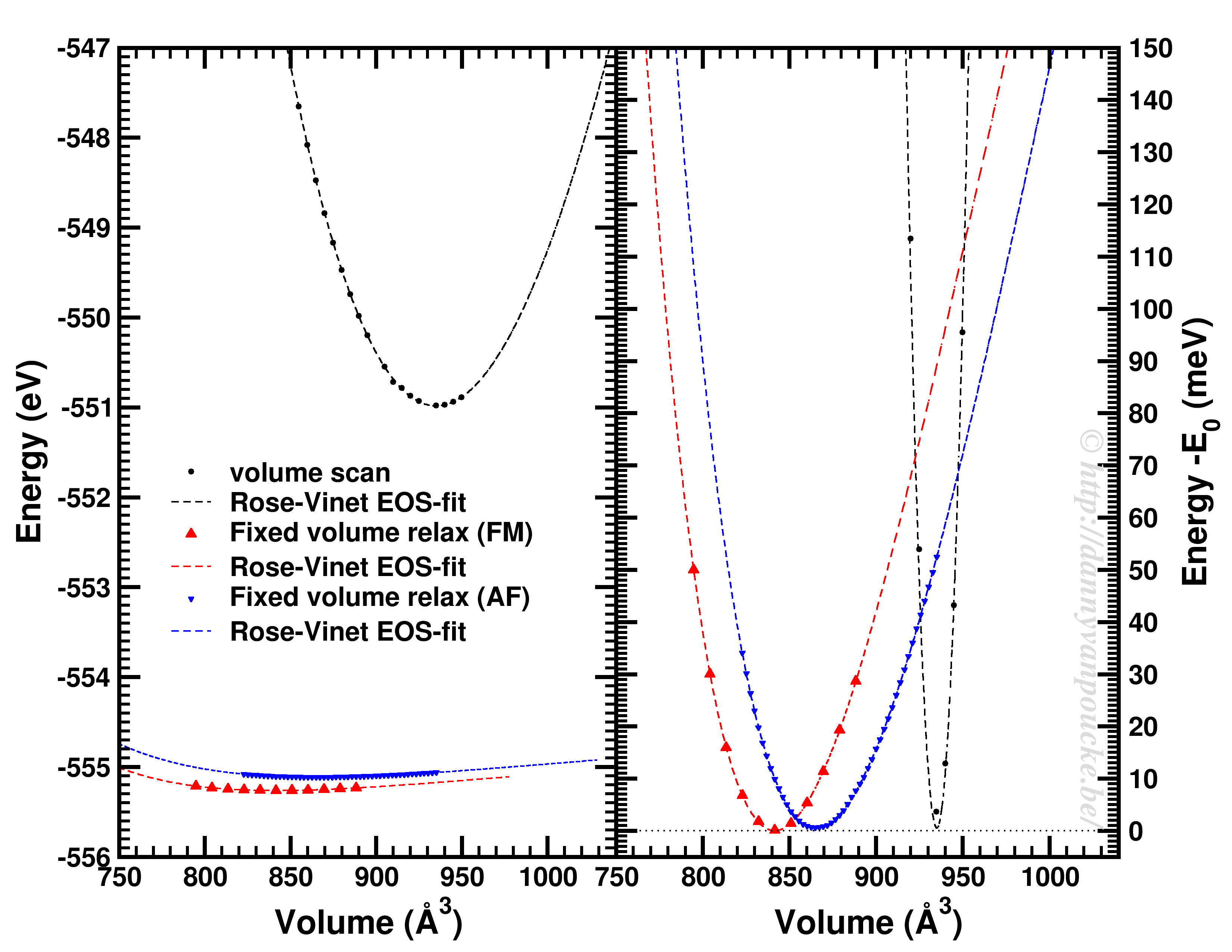
Comparison of a volume scan and an EOS-fit to fixed volume optimizations for a Metal-Organic Framework with MIL53/47 topology.
We just saw that for simple systems, the simple volume scan can already be too simple. For more complex systems like MOFs, similar problems can be seen. The simple volume scan, as for graphite gives a too sharp potential (with a very large bulk modulus). In addition, internal reordering of the atoms gives rise to very large changes in the energy, and the equilibrium volume can move quite a lot. It even depends on the spin-configuration.
In conclusion: the safest way to get a good equilibrium volume is unfortunately also the most expensive way. By means of an equation of state fit to a set of fixed volume structure optimizations the ground state (experimental) equilibrium volume can be found. As a bonus, the bulk modulus is obtained as well.
Permanent link to this article: https://dannyvanpoucke.be/vasp-tutor-eosfit-en/
Jan 01 2017
2016 has come and gone. 2017 eagerly awaits getting acquainted. But first we look back one last time, trying to turn this into a tradition. What have I done during the last year of some academic merit.
Publications: +4
Completed refereeing tasks: +5
Conferences: +4 (Attended) & + 1 (Organized)
PhD-students: +2
Current size of HIVE:
Hive-STM program:
Permanent link to this article: https://dannyvanpoucke.be/review-of-2016-en/
Dec 26 2016
When running programs on HPC infrastructure, one of the first questions to ask yourself is: “How well does this program scale?“
In applications for HPC resources, this question plays a central role, often with the additional remark: “But for your specific system!“. For some software packages this is an important remark, for other packages this remark has little relevance, as the package performs similarly for all input (or for given classes of input). The VASP package is one of the latter. For my current resource application at the Flemish TIER-1 I set out to do a more extensive scaling test of the VASP package. This is for 2 reasons. The first being the fact that I will be using a newer version of VASP: vasp 5.4.1 (I am currently using my own multiply patched version 5.3.3.). The second being the fact that I will be using a brand new TIER-1 machine (second Flemish TIER-1, as our beloved muk retired the end of 2016).
Why should I put in the effort to get access to resources on such a TIER-1 supercomputer? Because such machines are the life blood of the computational materials scientist. They are their sidekick in the quest for understanding of materials. Over the past 4 years, I was granted (and used) 20900 node-days of calculation time (i.e. over 8 Million hours of CPU time, or 916 years of calculation time) on the first TIER-1 machine.
Now back to the topic. How well does VASP 5.4.1 behave? That depends on the system at hand, and how good you choose the parallelization settings.
VASP provides several parameters which allow for straightforward parallelization of the simulation:
In addition, one needs to keep the architecture of the HPC-system in mind as well: NPAR, KPAR and their product should be divisors of the number of nodes (and cores) used.
Both NPAR and KPAR parameters can be set simultaneously and will have a serious influence on the speed of your calculations. However, not all possible combinations give the same speedup. Even worse, not all combinations are beneficial with regard to speed. This is best seen for a small 2 atom diamond primitive cell.
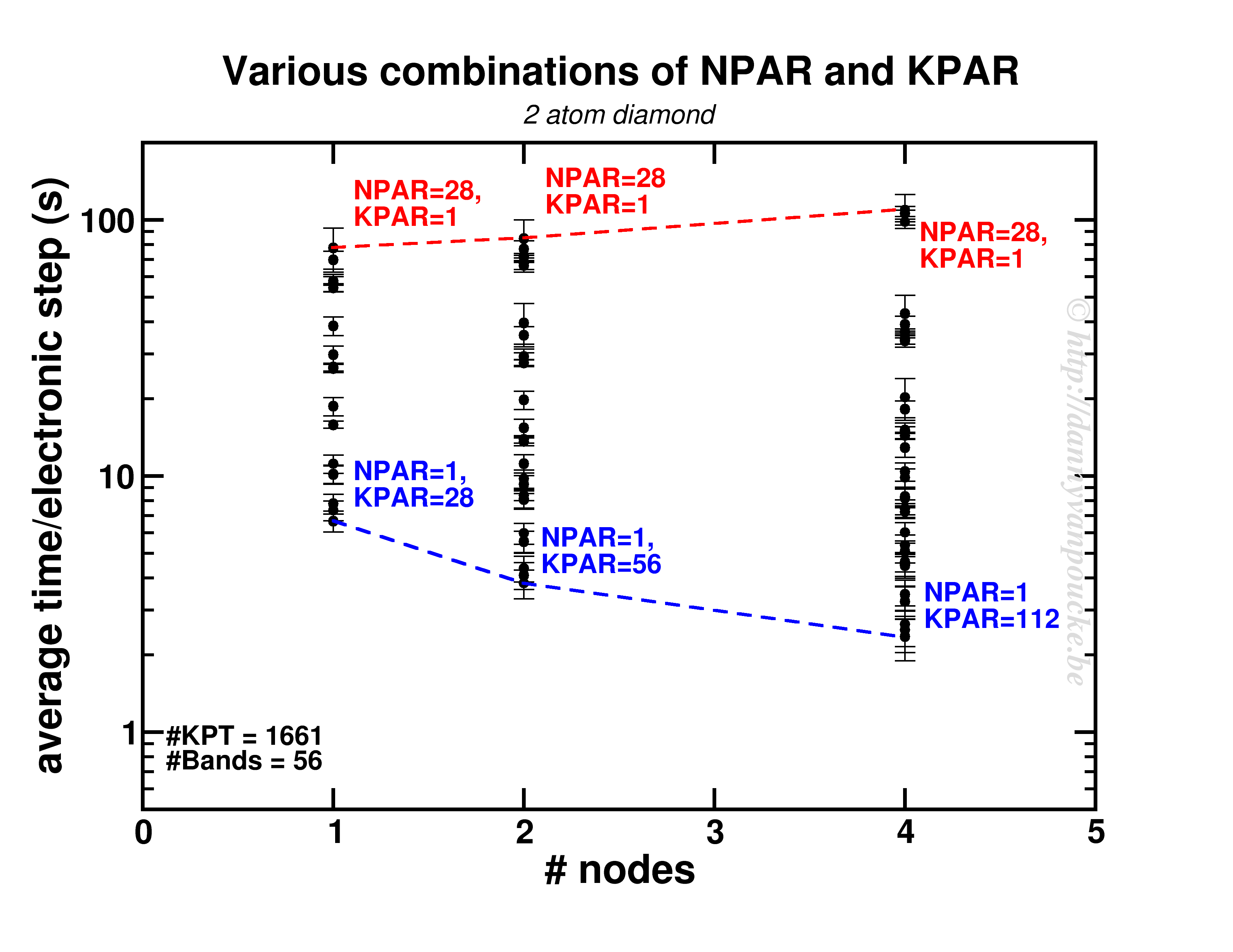
Timing results for various combinations of the NPAR and KPAR parameters for a 2 atom primitive unit cell of diamond.
Two things are clear. First of all, switching on a parallelization parameter does not necessarily mean the calculation will speed up. In some case it may actually slow you down. Secondly, the best and worst performance is consistently obtained using the same settings. Best: KPAR = maximal, and NPAR = 1, worst: KPAR = 1 and NPAR = maximal.
This small system shows us what you can expect for systems with a lot of k-points and very few electronic bands ( actually, any real calculation on this system would only require 8 electronic bands, not 56 as was used here to be able to asses the performance of the NPAR parameter.)
In a medium sized system (20-100 atoms), the situation will be different. There, the number of k-points will be small (5-50) while the natural number of electronic bands will be large (>100). As a test-case I looked at my favorite Metal-Organic Framework: MIL-47(V).
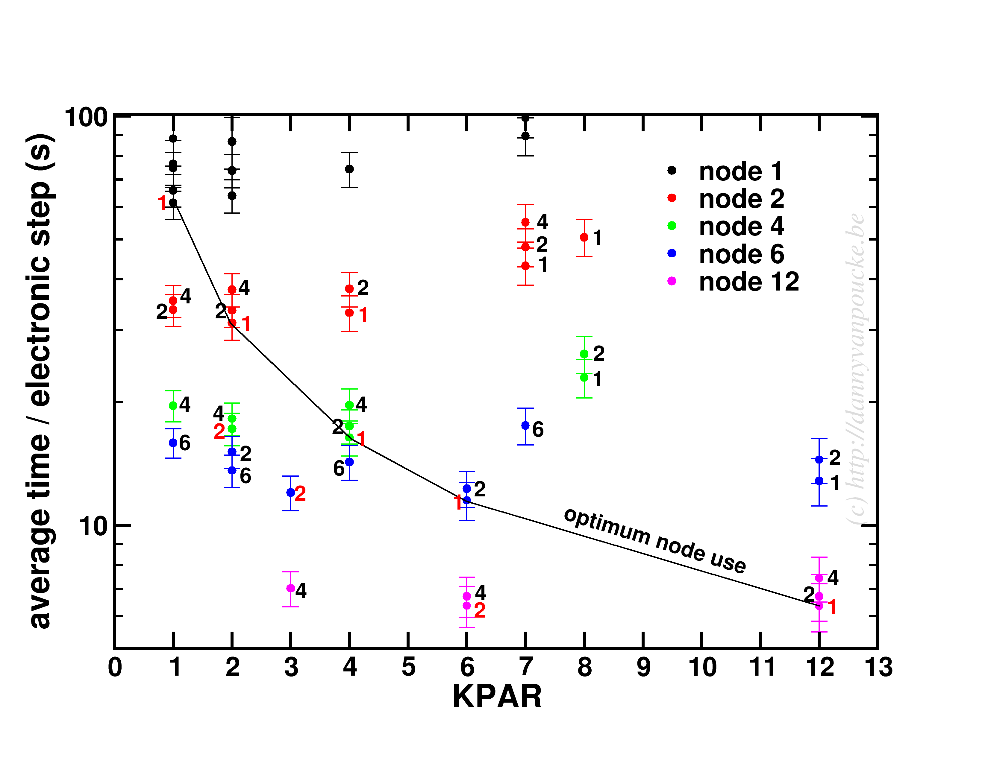
Timing results for several NPAR/KPAR combinations for the MIL-47(V) system.
This system has only 12 k-points to parallelize over, and 224 electronic bands. The spread per number of nodes is more limited than for the small system. In contrast, the general trend remains the same: KPAR=high, NPAR=low, with an optimum performance when KPAR=#nodes. Going beyond standard DFT, using hybrid functionals, also retains the same picture, although in some cases about 10% performance can be gained when using one half node per k-point. Unfortunatly, as we have very few k-points to start from, this will only be an advantage if the limiting factor is the number of nodes available.
An interesting behaviour is seen when one keeps the k-points/#nodes ratio constant:
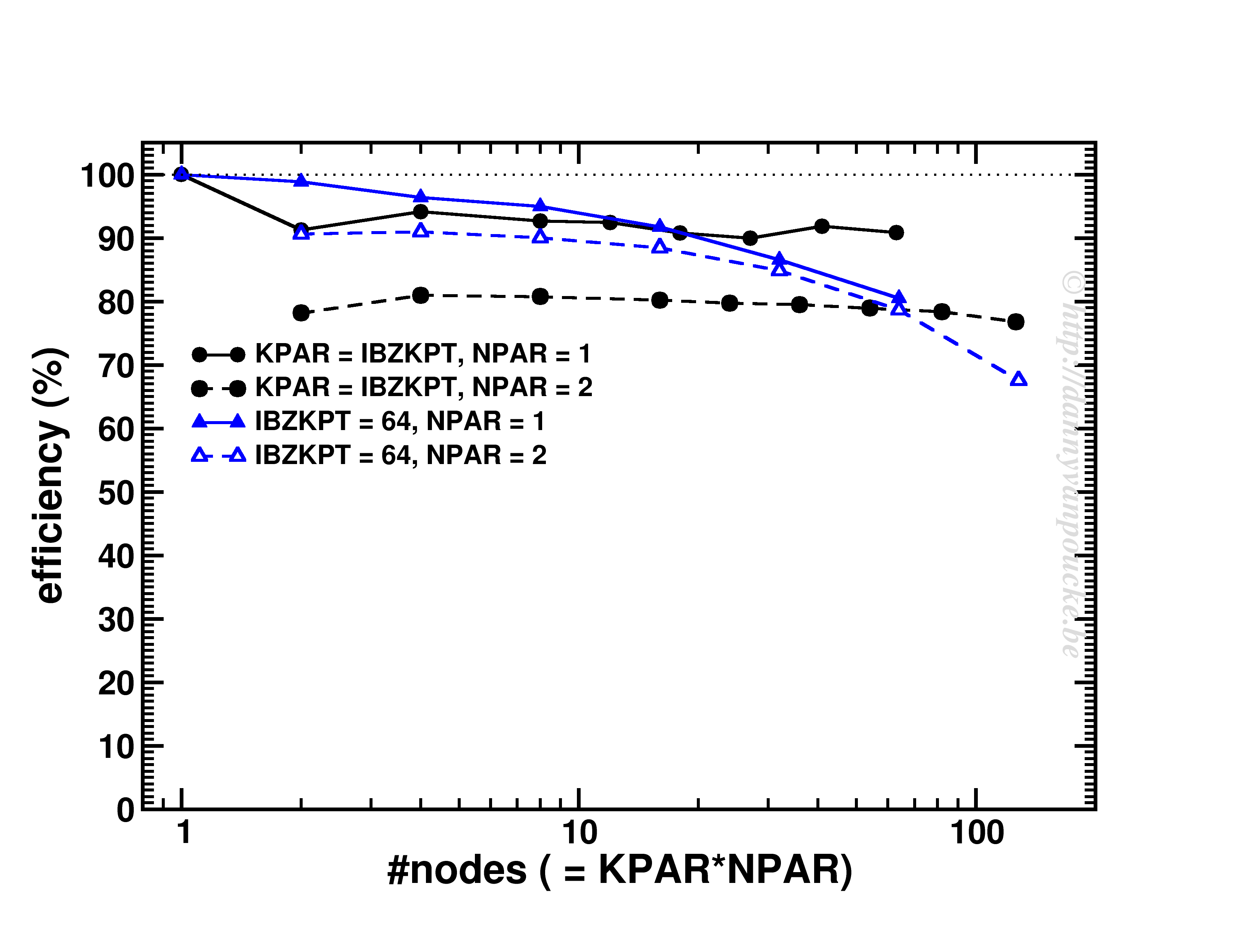
Scaling behavior for either a constant number of k-points (for dense k-point grid in medium sized system) or constant k-point/#nodes ratio.
As you can see, VASP performs really well up to KPAR=#k-points (>80% efficiency). More interestingly, if the k-point/#node ratio is kept constant, the efficiency (now calculated as T1/(T2*NPAR) with T1 timing for a single node, and T2 for multiple nodes) is roughly constant. I.e. if you know the walltime for a 2-k-point/2-nodes job, you can use/expect the same for the same system but now considering 20-k-points/20-nodes (think Density of States and Band-structure calculations, or just change of #k-points due to symmetry reduction or change in k-point grid.) 😆
If one thing is clear from the current set of tests, it is the fact that good scaling is possible. How it is attained, however, depends greatly on the system at hand. More importantly, making a poor choice of parallelization settings can be very detrimental to the obtained speed-up and efficiency. Unfortunately when performing calculations on an HPC system, one has externally imposed limitations to work with:
Here are some guidelines (some open doors as well):
In short:
[1] 28 is a lousy number in that regard as its prime-decomposition is 2x2x7, leaving little overlap with prime-decompositions of the number of k-points, which more often than you wish end up being prime numbers themselves 😥
[2] The small system’s memory requirements varied from 0.15 to 1.09 Gb/core for the different combinations.
Permanent link to this article: https://dannyvanpoucke.be/scaling-vasp-breniac-en/
Dec 21 2016

Black arts of computational materials science.
Today the projects for the third year bachelor students in physics were presented at UHasselt. I also contributed two projects, giving the students the opportunity to choose for a computational materials science project. During these projects, I hope to introduce them into the modern (black) arts of High-Performance Computing and materials modelling beyond empirical models.
The two projects focus each on a different aspect of what it is to be a computational materials scientist. One project focuses on performing quantum mechanical calculations using the VASP program, and analyzing the obtained results with existing software. This student will investigate the NV-defect complex in diamond in all its facets. The other project focuses on the development of new tools to investigate the data generated by simulation software like VASP. This student will extend the existing phonon module in the HIVE-toolbox and use it to analyse a whole range of materials, varying from my favourite Metal-Organic Framework to a girl’s best friend: diamond.
Calculemus solidi
A description of the projects in Dutch can be found here.
Permanent link to this article: https://dannyvanpoucke.be/baproj2017-en/
Dec 20 2016
One of the main differences between theory and computational research is the fact that the latter has to deal with finite resources; mainly time and storage. Where theoretical calculations involve integrations over continuous spaces, infinite sums and basis sets, computational work performs numerical integrations as weighted sums over finite grids and cuts of infinite series. As an infinite number of operations would take an infinite amount of time, it is clear why numerical evaluations are truncated. If the contributions of an infinite series become smaller and smaller, it is also clear that at some point the contributions will become smaller than the numerical accuracy, so continuation beyond that point is …pointless.
In case of ab initio quantum mechanical calculations, we aim to get as accurate results at an as low computational cost as possible. Even with the current availability of computational resources, an infinite sum would still take an infinite amount of time. In addition, although parallelization can help out a lot in getting access to additional computational resources during the same amount of real time, codes are not infinitely parallel, so at some point adding more CPU’s will no longer speed up the calculations. Two important parameters in quantum mechanical calculations to play with are the basis set size (Or kinetic energy cut off, in case of plane wave basis sets. In which case this can also be related to the real space integration grid) and the integration grid for the reciprocal space (the k-point grid).
These two parameters are not unique to VASP, they are present in all quantum mechanical codes, but we will use VASP as an example here. The example system we will use is the α-phase of Cerium, using the PBE functional. The default cut-off energy used by VASP is 299 eV.
What a basis set is and how it is defined depends strongly on the code. As such you are referred to the manual/tutorials of your code of interest.(VASP workshop) One important thing to remember, however, is the fact that although a plane wave basis set is “nicely behaved” (bigger basis = more accurate result) this is not true for all types of basis sets (Gaussian basis sets are an important example here).
How do you perform a convergence test?
This does not need to be a fully optimized geometry, an experimental geometry or a reasonable manually constructed geometry will do fine, as long as it gives you a converged result at the end of your static calculation. A convergence test should not depend on the exact geometry of your system. Rather it should tell you how well your setting converges your result with regard to the energy found on the potential energy surface.
(to reasonable values, although the settings should—to make your life somewhat sane—be independent with regard to convergence testing).
VASP specific parameters of importance:
These should be a simple static calculation. Make sure that each of the calculations finishes successfully, otherwise you will not be able to compare results and check convergence.
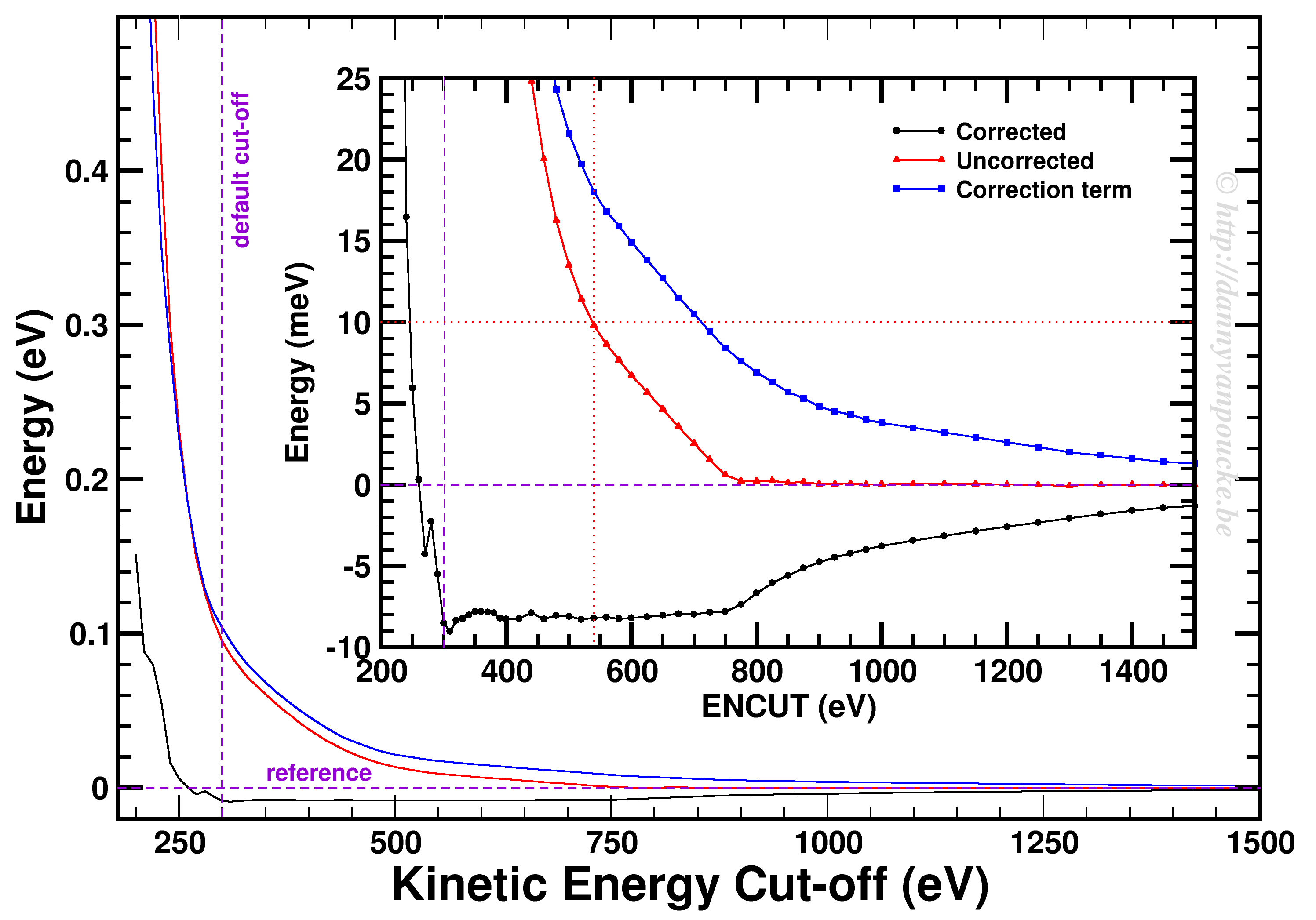
Convergence of the kinetic energy cut-off for alpha Ce using the PBE functional and a 9x9x9 k-point grid.
In our example, we used a 9x9x9 k-point set. Looking at the example, we first of all see how smoothly the total energy varies with regard to the ENCUT parameter. In addition, it is important to note that VASP has a correction term (search for EATOM in the OUTCAR file) implemented which greatly improves the energy convergence (compare the black and red curves). Unfortunately, it also leads to non-variational convergence (i.e. the energy does not become strictly smaller with increasing cut-off) which may lead to some confusion. However, the correction term performs really well, and allows you to use a kinetic energy cut-off which is much lower than what you would need to use without. In this case, the default cut-off misses the reference energy by about 10 meV. Without the correction, a cut-off of about 540 eV (almost double) is needed. From ENCUT=300 to 800 eV, you observe a plateau, so using a higher cut-off will not improve the energy much. However, other properties, such as the calculated forces or the hessian may improve in this region. For these parameters a higher cut-off may be beneficial, and their convergence as function of ENCUT should be checked if important for your work.
Similar as for the kinetic energy cut-off, if you are working with a periodic system you should check the convergence of your k-point set. However, if you are working with molecules/clusters your Brillouin zone reduces to a single point, so your k-point set should only consist of the Gamma point and no convergence testing is needed. More importantly, if you use a larger k-point set for such systems (molecules/clusters) you introduce artificial interaction between the periodic copies which should be avoided at all cost.
For bulk materials a k-point convergence check has a similar setup as the basis set convergence check. The main difference being the fact that for these calculation the basis set is kept constant (VASP: ENCUT = default cut-off, manually set) and the k-point set is varied. As such, if you are new to quantum mechanical calculations, or start using a new code, you can combine the two convergence checks and study the convergence behavior on a 2D surface.
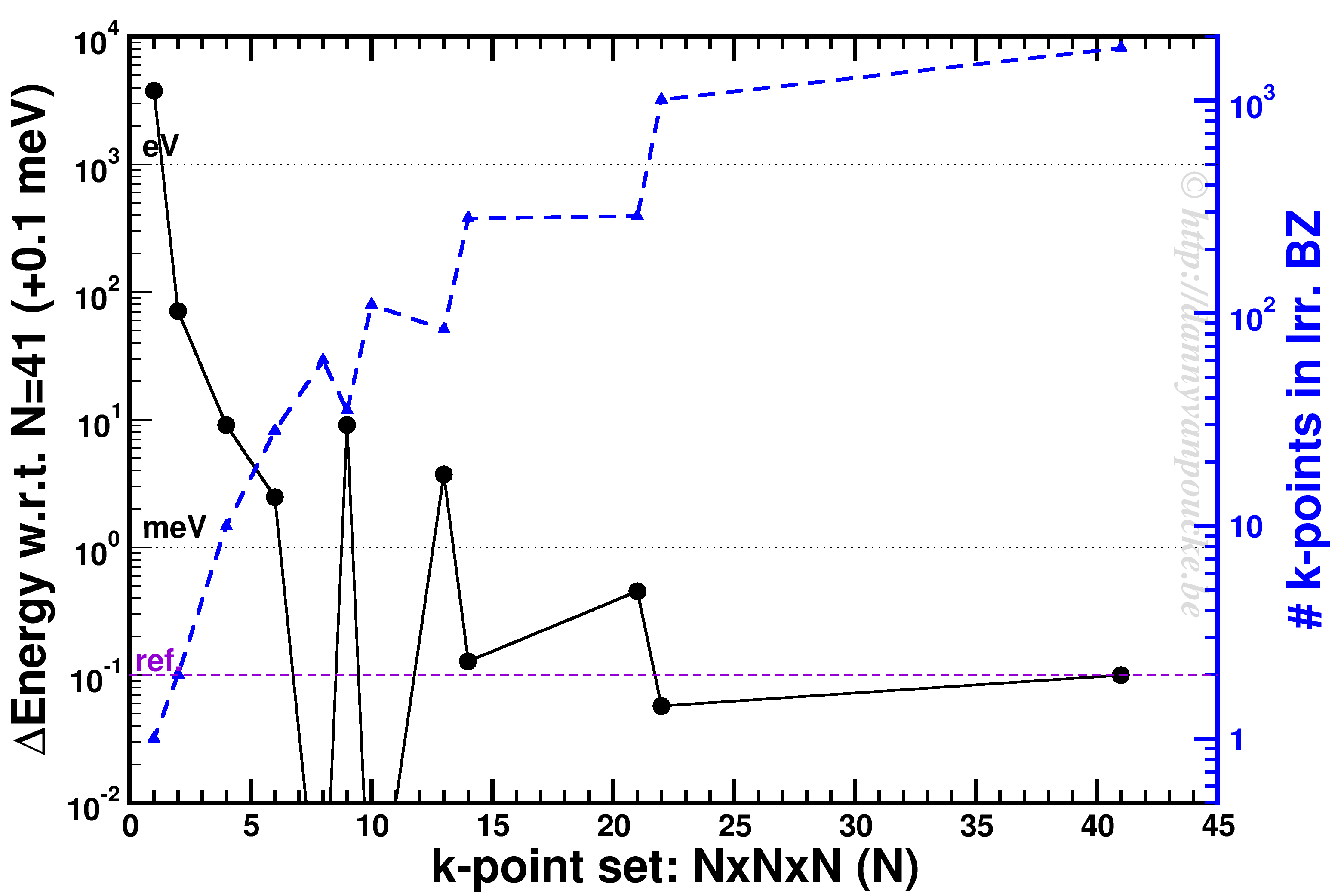
K-point convergence of alpha-Cerium using the PBE functional and ENCUT=500 eV.
In our example, ENCUT was set to 500 eV. It is clear that an extended k-point set is important for small systems, as the Gamma-point only energy can be off by several eV. This is even the case for some large systems like MOFs. An important thing to remember with regard to k-point convergence, is the fact that this convergence is not strictly declining, it may show significant oscillations overshooting and undershooting the converged value. A convergence of 1 meV or less for the entire system is a goal to aim for. An exception may be the most large systems, but even then one should keep in mind the size of the energy barriers in that system. Using flexible MOFs as an example which show a large-pore to narrow-pore transition barrier of 10-20 meV per formula unit, k-point convergence should be much below this. Otherwise your system may accidentally cross this barrier during relaxation.
The blue curve shows the number of k-points in the irreducible Brillouin zone. For standard density functional theory calculations (LDA and GGA, not hybrid functionals) this is a measure of the computational cost, as the k-points can be calculated fully independently in parallel (and yes the blue scale is a log-scale as well). Because the first orders of magnitude in accuracy are quickly crossed ( from Gamma to 6x6x6 the energy error goes from the order of eV to meV) while the number of k-points doesn’t grow that quickly (from 1 to 28). As a result, one often performs structure optimizations in a stepped fashion, starting with a coarse grid steadily increasing the grid (unless pathological behavior is expected… MOFs again…yes, they do leave you with nightmares in this regard).
Convergence testing is necessary, in theory, for each and every new system you look into. Luckily, VASP behaves rather nicely, such that over time you will know what to expect and your convergence tests will reduce in size significantly and become more focused. In the examples above we used the total energy as a reference, but this is not always the most important aspect to consider. In some cases you should check the convergence as function of the accuracy of the forces. In that case you generally will end up with more stringent criteria as energy converges rather nicely and quickly.
May your convergence curves be smooth and quick.
Permanent link to this article: https://dannyvanpoucke.be/vasp-tutor-convergence-testing-en/
Dec 13 2016
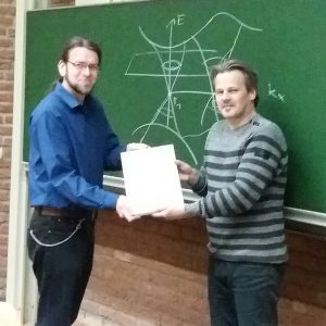
Bart Sorée receives a commemorative frame of the event. Foto courtesy of Rajesh Ramaneti.
Today I have the pleasure of chairing the last symposium of the year of the MRS chapter at UHasselt. During this invited lecture, Bart Sorée (Professor at UAntwerp and KULeuven, and alumnus of my own Alma Mater) will introduce us into the topic of topological insulators.
This topic became unexpectedly a hot topic as it is part of the 2016 Nobel Prize in Physics, awarded last Saturday.
This year’s Nobel prize in physics went to: David J. Thouless (1/2), F. Duncan M. Haldane (1/4) and J. Michael Kosterlitz (1/4) who received it
On the Nobel Prize website you can find this document which gives some background on this work and explains what it is. Beware that the explanation is rather technical and at an abstract level. They start with introducing the concept of an order parameter. You may have heard of this in the context of dynamical systems (as I did) or in the context of phase transitions. In the latter context, order parameters are generally zero in one phase, and non-zero in the other. In overly simplified terms, one could say an order parameter is a kind of hidden variable (not to be mistaken for a hidden variable in QM) which becomes visible upon symmetry breaking. An example to explain this concept.
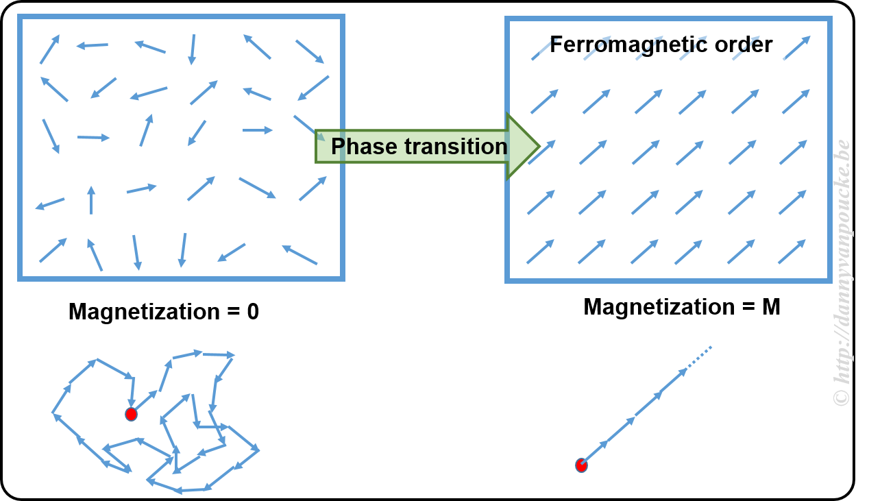
In a ferromagnetic material, the atoms have what is called a spin (imagine it as a small magnetic needle pointing in a specific direction, or a small arrow). At high temperature these spins point randomly in all possible directions, leading to a net zero magnetization (the sum of all the small arrows just lets you run in circles going nowhere). This magnetization is the order parameter. At the high temperature, as there is no preferred direction, the system is invariant under rotation and translations (i.e. if you shift it a bit or you rotate it, or both you will not see a difference) When the temperature is lower, you will cross what is called a critical temperature. Below this temperature all spins will start to align themselves parallel, giving rise to a non-zero magnetization (if all arrows point in the same direction, their sum is a long arrow in that direction). At this point, the system has lost the rotational invariance (because all spins point in direction, you will know when someone rotated the system) and the symmetry is said to have broken.
Within the context of phase transitions, order parameters are often temperature dependent. In case of topological materials this is not the case. A topological material has a topological order, which means both phases are present at absolute zero (or the temperature you will never reach in any experiment no matter how hard you try) or maybe better without the presence of temperature (this is more the realm of computational materials science, calculations at 0 Kelvin actually mean without temperature as a parameter). So the order parameter in a topological material will not be temperature dependent.
To complicate things, topological insulators are materials which have a topological order which is not as the one defined above 😯 —yup why would we make it easy 🙄 . It gets even worse, a topological insulator is conducting.
OK, before you run away or loose what is remaining of your sanity. A topological insulator is an insulating material which has surface states which are conducting. In this it is not that different from many other “normal” insulators. What makes it different, is that these surface states are, what is called, symmetry protected. What does this mean?
In a topological insulator with 2 conducting surface states, one will be linked to spin up and one will be linked to spin down (remember the ferromagnetism story of before, now the small arrows belong to the separate electrons and exist only in 2 types: pointing up=spin up, and pointing down=spin down). Each of these surface states will be populated with electrons. One state with electrons having spin up, the other with electrons having spin down. Next, you need to know that these states also have a real-space path let the electrons run around the edge of material. Imagine them as one-way streets for the electrons. Due to symmetry the two states are mirror images of one-another. As such, if electrons in the up-spin state more left, then the ones in the down-spin state move right. We are almost there, no worries there is a clue. Now, where in a normal insulator with surface states the electrons can scatter (bounce and make a U-turn) this is not possible in a topological insulator. But there are roads in two directions you say? Yes, but these are restricted. And up-spin electron cannot be in the down-spin lane and vice versa. As a result, a current going in such a surface state will show extremely little scattering, as it would need to change the spin of the electron as well as it’s spatial motion. This is why it is called symmetry protected.
If there are more states, things get more complicated. But for everyone’s sanity, we will leave it at this. 😎
Permanent link to this article: https://dannyvanpoucke.be/topological-insulators-en/
Nov 23 2016
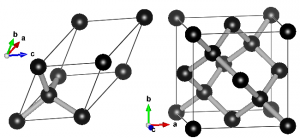
Ball-and-stick representation of diamond in two different unit cells. Left: primitive unit cell containing two atoms. All atoms at the vertices are periodic copies of the same one. Right: Conventional cubic unit cell containing eight atoms. Atoms at opposing faces are periodic copies, while all atoms at the vertices are periodic copies of the same atom.
When performing electronic structure calculations on complex systems, you prefer to do this on systems with as few atoms as possible. Such periodic cells are called unit cells. There are, however, two types of unit cells: Primitive unit cells and conventional unit cells.
A primitive unit cell is the smallest possible periodic cell of a crystalline material, making it extremely suited for calculations. Unfortunately, it is not always the nicest unit cell to work with, as it may be difficult to recognize it’s symmetry (cf. the example of diamond on the right). The conventional unit cell on the other hand shows the symmetry more clearly, but is not (always) the smallest possible unit cell. To make matters complicated and confusing, people often refer to both types as simply “unit cell”, which is not wrong, but the term unit cell is for many uniquely associated with only one of the two types.
When you are performing calculations on diamond, the conventional cell isn’t that large that standard calculations become impossible, even on a personal laptop or desktop. On the other hand, when you are studying a Metal-Organic Framework like the UiO-66(Zr) which contains 456 atoms in its conventional unit cell, you will be very happy to use the primitive unit cell with ‘merely’ 114 atoms. Also the MIL-47/53 topology which generally is studied using a conventional unit cell containing 72/76 can be reduced to a smaller primitive unit cell of only 36/38 atoms. Just as for the diamond primitive unit cell, this MIL47/53 primitive unit cell is not a nice cubic cell. Instead you end up with a lattice having lattice angles of seventy-something degrees.
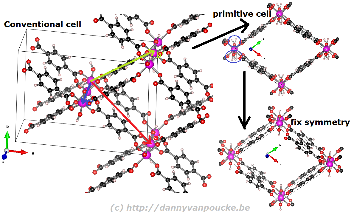
Reduction of the MIL-53 conventional cell to the primitive cell. The conventional cell is shown, extending slightly into the periodic copies. The primitive lattice vectors are shown as colored arrows. The folded primitive cell shows there was some symmetry-breaking in the hydroxy groups of the metal-oxide chain. Introducing some additional symmetry fixes this in the final primitive cell.
Before you start, and if you are using VASP, make sure you have the POSCAR file giving the atomic positions as Cartesian coordinates. (Using the HIVE-4 toolbox: Option TF, suboption 2 (Dir->Cart).)
If you do not use VASP, you can still make use of the scheme below.
 |
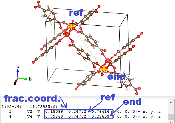 |
⇒ aprim = axprim,frac aconv + ayprim,frac bconv + azprim,frac cconv
So imagine that the lattice vectors of the MOF above are a = ( 20, 0, 0), b = ( 0, 15, 0), and c = ( 0, 0, 5). And the primitive fractional a vector is found to be aprim,frac = ( 0.5, -0.5, 0.5). In this case the aprim vector will become: aprim = ( 10, 0, 0 ) + ( 0, -7.5, 0 ) + ( 0, 0, 2.5) = (10, -7.5, 2.5).
As you can see, the method is quite simple and straight forward, albeit a bit tedious if you need to do this many times.
PS: Small remark for those new to VESTA. You can use delete atoms in VESTA and store your structure again. This is useful if you want to play with a molecule. Unfortunately for a solid you need also to get new lattice vectors, which did not happen. As a result you end up with some atoms floating around in a periodically repeated box with the original lattice parameters. Steps 1-5 given above provide a simple way of not ending up in this situation, but require some typing on your part.
PS 2: The opposite transformation, from a primitive unit cell to a conventional unit cell, using VESTA, is shown in this youtube video.
Permanent link to this article: https://dannyvanpoucke.be/vasp-tutor-creating-a-unit-cell-from-a-super-cell-en/
Nov 16 2016
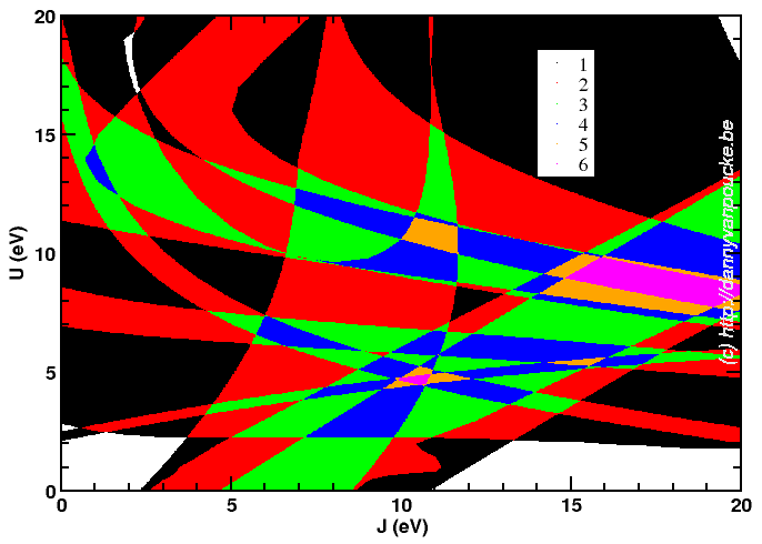
Although it looks a bit like a modern piece of art, it is one more attempt at trying to find an optimum combination of parameters.
I’m currently trying to find “the best choice” for U and J for a DFT+U based project… DFT??? Density Functional Theory. This is an approximate method which is used in computational materials science to calculate the quantum mechanical behavior of electrons in matter. Instead of solving the Schrödinger equation, known from any quantum mechanic course, one solves the Hohenberg-Kohn-Sham equations. In these equations it are not the electrons which play a central role (which they do in the Schrödinger equations) but the electron density. Hohenberg, Kohn and Sham were able to show that their equations give the exact same results as the Schrödinger equations. There is, however, one small caveat: you need to have an “exact” exchange-correlation functional (a functional is just a function of a function). Unfortunately there is no known analytic form for this functional, so one needs to use approximated functionals. As you probably guessed, with these approximate functionals the solution of the Hohenberg-Kohn-Sham equations is no longer an exact solution.
For some molecules or solids the error is much larger than average due to the error in the exchange-correlation functional. These systems are therefore called “strongly-correlated” systems. Over the years, several ways have been devised to solve this problem in DFT. One of them is called DFT+U. It entails adding additional coulomb interactions (Hubbard-U-potential) between the “strongly interacting electrons”. However this additional interaction depends on the system at hand, so one always needs to fit this parameter against one of more properties one is interested in. The law of conservation of misery, however, makes sure that improving one property goes hand in hand with a deterioration of another property.
Since actual DFT+U has two independent parameters (U and J, though for many systems they can be dependent reducing to a single parameter) I had quite some fun running calculations for a 21×21 grid of possible pairs. Afterward, collecting the data I wanted to use for fitting purposes took my script about 2h! 😯 Unfortunately the 10 properties of interest I wanted to fit give optimum (U,J)-pair all over the grid. In the picture above, you see my most recent attempt at trying to deal with them. It shows for the entire grid how many of the 10 properties are reasonably well fit.There are two regions which fit 6 properties; One around (U,J)=(5,10) and another around (U,J)=(8.5,17.5). There will be more work before this gives a satisfactory result, the show will go on.
Permanent link to this article: https://dannyvanpoucke.be/modern-art-in-research-en/
Oct 18 2016
 Yesterday was a good day for computational scientists in Flanders. The new TIER-1 machine, named BrENIAC, located at the university of Leuven, was inaugurated and is now officially open to all users of the Flemish university associations: UAntwerpen, VUB, UGhent, UHasselt, and KULeuven. The name refers to one of the first (super)computers ever built: ENIAC. This new machine will take over the task of the first TIER-1 machine (muk, located at the university of Ghent), which will be decommissioned at the end of this year. BrENIAC is ranked 196th in the current top 500 of supercomputers, and costs 5.5 M€. This is of course without the annual cost of power usage and technical personnel which will maintain the machine and provide support for the scientists running calculations. With its 580 compute nodes, containing 28 cores each (or 2 14-core CPU’s of the type Broadwell E5-2680v4), the number of available cores has roughly doubled. Also memory access should have improved, which gives rise to a theoretical threefold increase of the peak performance.
However, this peak performance is measured with “benchmark” tests, which tend to behave much better than real life programs. This is because the average scientific programmer doesn’t write the best optimized code (ok, “commercial” programs these days may even behave worse :p ) for various reasons, time constraints being one of them. So my first task, before I start running my simulations on the new TIER-1 machine, will be to benchmark VASP and my own HIVE-code.
Two videos of my new sidekick:
You can see me in my front-row position in this picture taken during the non-academic part of the inauguration.
Permanent link to this article: https://dannyvanpoucke.be/breniac-en/