Most commented posts
- Start to Fortran — 1 comment
- Phonons: shake those atoms — 3 comments


Jun 16 2017
This semester I had several teaching assignments. I was a TA for the course biophysics for the first bachelor biomedical sciences, supervised two 3rd bachelor students physics during their first steps in the realm of computational materials science, and finally, I was responsible for half the course Functional Molecular Modelling for the first Masters Biomedical students (Bioelectronics and Nanotechnology). In this course, I introduce the the students into the basic concepts of classical molecular modelling (quantum modelling is covered by Prof. Wilfried Langenaeker). It starts with a reiteration of some basic concepts from statistics and moves on to cover the canonical ensemble. Things get more interesting with the introduction into Monte-Carlo(MC) and Molecular Dynamics(MD), where I hope to teach the students the basics needed to perform their own MC and MD simulations. This also touches the heart of what this course should cover. If I hear a title like Functional Molecular Modelling, my thoughts move directly to practical applications, developing and implementing models, and performing simulations. This becomes a bit difficult as none of the students have any programming experience or skills.
Luckily there is excel. As the basic algorithms for MC and MD are actually quite simple, this office package can be (ab)used to allow the students to perform very simple simulations. This even without the use of macro’s or any advanced features. Because Excel can also plot the data present in the cells, you immediately see how properties of the simulated system vary during the simulation, and you get direct update of all graphs every time a simulation is run.
It seems I am not the only one who is using excel for MD simulations. In 1995, Fraser and Woodcock even published a paper detailing the use of excel for performing MD simulations on a system of 100 particles. Their MD is a bit more advanced than the setup I used as it made heavy use of macro’s and needed some features to speed things up as much as possible. With the x486 66MHz computers available at that time, the simulations took of the order of hours. Which was impressive, as they served as an example of how computational speed had improved over the years, and compared to the months of supercomputer resources one of the authors had needed 25 years earlier to perform the same thing for his PhD. Nowadays the same excel simulation should only take minutes, while an actual program in Fortran or C may even execute the same thing in a matter of seconds or less.
For the classes and exercises, I made use of a simple 3-atom toy-model with Lennard-Jones interactions. The resulting simulations remain clear allowing their use for educational purposes. In case of MC simulations, a nice added bonus is the fact that excel updates all its fields automatically when a cell is modified. As a result, all random numbers are regenerated and a new simulation can be performed by saving the excel-sheet or just modifying a not-used cell.
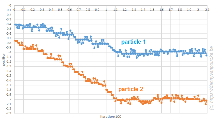
Monte Carlo in excel. A system of three particles on a line, with one particle fixed at 0. All particles interact through a Lennard-Jones potential. The Monte Carlo simulation shows how the particles move toward their equilibrium position.
The simplicity of Newton’s equations of motion make it possible to perform simple MD simulations, and already for a three particle system, you can see how unstable the algorithm is. Implementation of the leap-frog algorithm isn’t much more complex and shows incredible the stability of this algorithm. In the plot of the total energy you can even see how the algorithm fights back to retain stability (the spikes may seem large, but the same setup with a straight forward implementation of Newton’s equation of motion quickly moves to energies of the order of 100).
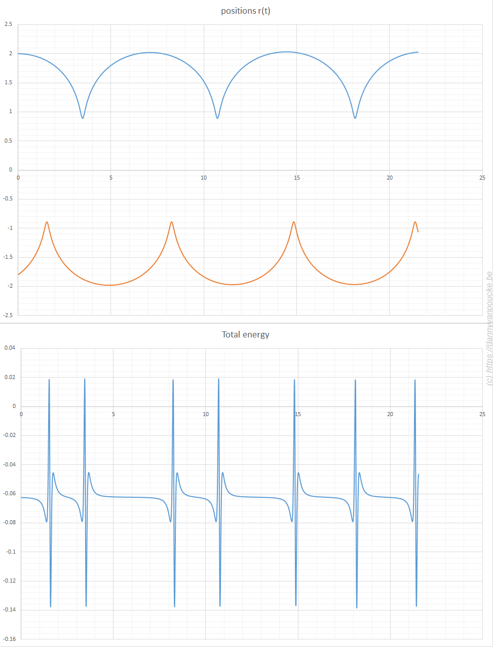
Molecular dynamics in excel. A system of three particles on a line, with one particle fixed at 0. All particles interact through a Lennard-Jones potential. The Molecular dynamics simulation shows how the particles move as time evolves. Their positions are updated using the leap-frog algorithm. The extreme hard nature of the Lennard-Jones potential gives rise to the sharp spikes in the total energy. It is this last aspect which causes the straight forward implementation of Newton’s equations of motion to fail.
Permanent link to this article: https://dannyvanpoucke.be/functional-molecular-modelling-simulating-particles-in-excel/
Jun 09 2017

Black arts of computational materials science.
Just over half a year ago, I mentioned that I presented two computational materials science related projects for the third bachelor physics students at the UHasselt. Both projects ended up being chosen by a bachelor student, so I had the pleasure of guiding two eager young minds in their first steps into the world of computational materials science. They worked very hard, cursed their machine or code (as any good computational scientist should do once in a while, just to make sure that he/she is still at the forefront of science) and survived. They actually did quite a bit more than “just surviving”, they grew as scientists and they grew in self-confidence…given time I believe they may even thrive within this field of research.
One week ago, they presented their results in a final presentation for their classmates and supervisors. The self-confidence of Giel, and the clarity of his story was impressive. Giel has a knack for storytelling in (a true Pan Narrans as Terry Pratchett would praise him). His report included an introduction to various topics of solid state physics and computational materials science in which you never notice how complicated the topic actually is. He just takes you along for the ride, and the story unfolds in a very natural fashion. This shows how well he understands what he is writing about.
This, in no way means his project was simple or easy. Quite soon, at the start of his project Giel actually ran into a previously unknown VASP bug. He had to play with spin-configurations of defects and of course bumped into a hand full of rookie mistakes which he only made once *thumbs-up*. (I could have warned him for them, but I believe people learn more if they bump their heads themselves. This project provided the perfect opportunity to do so in a safe environment. 😎 ) His end report was impressive and his results on the Ge-defect in diamond are of very good quality.
The second project was brought to a successful completion by Asja. This very eager student actually had to learn how to program in fortran before he could even start. He had to implement code to calculate partial phonon densities with the existing HIVE code. Along the way he also discovered some minor bugs (Thank you very much 🙂 ) and crashed into a rather unexpected hard one near the end of the project. For some time, things looked very bleak indeed: the partial density of equivalent atoms was different, and the sum of all partial densities did not sum to the total density. As a result there grew some doubts if it would be possible to even fulfill the goal of the project. Luckily, Asja never gave up and stayed positive, and after half a day of debugging on my part the culprit was found (in my part of the code as well). Fixing this he quickly started torturing his own laptop calculating partial phonon densities of state for Metal-organic frameworks and later-on also the Ge-defect in diamond, with data provided by Giel. Also these results are very promising and will require some further digging, but they will definitely be very interesting.
For me, it has been an interesting experience, and I count myself lucky with these two brave and very committed students. I wish them all the best of luck for the future, and maybe we meet again.
Permanent link to this article: https://dannyvanpoucke.be/bachelor-projects-completed/
Jun 07 2017
Last Friday, the HPC infrastructure in Flanders got celebrated by the VSC user day. Being one of the Tier-1 supercomputer users at UHasselt, I was asked if I could present a poster at the meeting, showcasing the things I do here. Although I was very interested in this event, educational obligations (the presentations of the bachelor projects, on which I will post later) prevented me from attending the meeting.
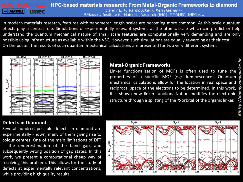
As means of a compromise, I created a poster for the meeting which Geert Jan Bex, our local VSC/HPC support team, would be so nice to put up at the event. The poster session was preceded by a set of 1-minute presentations of the posters, for which a slide had to be made. As I could not be physically present, I provided the organizers a slide which contained a short description that could be used as the 1-minute presentation. Unfortunately, things got a little mixed up, as Geert Jan accidentally printed this slide as the poster (which gave rise to some difficulties in the printing process 🙄 ). So for those who might have had an interest in the actual poster, let me put it up here:

This poster presents my work on linker functionalisation of the MIL-47, which got recently published in the Journal of physical chemistry C, and the diamond work on the C-vacancy, which is currently submitted. Clicking on the poster above will provide you the full size image. The 1-minute slide presentation, which erroneously got printed as poster:
Permanent link to this article: https://dannyvanpoucke.be/vsc-user-day-2017-the-poster-edition/
May 09 2017
With a recent transfer of this website to a new server, I was able to move it more or less entirely into the HTTPS domain. The main reason for doing this is the recent hobby of Google (and chrome as it’s extension) to target HTTP websites to indicate them as insecure [1,2,3]. The transfer from HTTP to HTTPS provides some security with regard to Man-In-The-middle attacks (or for those with the background in quantum information and quantum cryptography: it protects Alice and Bob from Eve…). It unfortunately will not protect my website from being hacked, nor you if I would include “evil” scripts into a page or post. 😈
Those who are interested in the “security” of this website may notice some pages are not yet labeled as secure. The origin lies in the sitemeter used to measure traffic. As it does not allow for an HTTPS connection to the used script. Other than that everything on the pages should be over HTTPS. The sole exceptions are some of the posts, which may still be using the HTTP version of the CSS style sheets and javascript scripts used to securely hide my email. If you notice something like this, feel free to put it in a comment under the post, and I’ll fix it as soon as possible.).
Permanent link to this article: https://dannyvanpoucke.be/improved-security-https/
Apr 28 2017
| Authors: | Seyyed Amin Rounaghi, Danny E.P. Vanpoucke, Hossein Eshghi, Sergio Scudino, Elaheh Esmaeili, Steffen Oswald and Jürgen Eckert |
| Journal: | Phys. Chem. Chem. Phys. 19, 12414-12424 (2017) |
| doi: | 10.1039/C7CP00998D |
| IF(2017): | 3.906 |
| export: | bibtex |
| pdf: | <Phys.Chem.Chem.Phys.> |
Nowadays, the development of highly efficient routes for the low cost synthesis of nitrides is greatly growing. Mechanochemical synthesis is one of those promising techniques which is conventionally employed for the synthesis of nitrides by long term milling of metallic elements under pressurized N2 or NH3 atmosphere (A. Calka and J. I. Nikolov, Nanostruct. Mater., 1995, 6, 409-412). In the present study, we describe a versatile, room-temperature and low cost mechanochemical process for the synthesis of nanostructured metal nitrides (MNs), carbonitrides (MCNs) and carbon nitride (CNx). Based on this technique, melamine as a solid nitrogen-containing organic compound (SNCOC) is ball milled with four different metal powders (Al, Ti, Cr and V) to produce nanostructured AlN, TiCxN1-x, CrCxN1-x, and VCxN1-x (x~0.05). Both theoretical and experimental techniques are implemented to determine the reaction intermediates, products, by-products and finally, the mechanism underling this synthetic route. According to the results, melamine is polymerized in the presence of metallic elements at intermediate stages of the milling process, leading to the formation of a carbon nitride network. The CNx phase subsequently reacts with the metallic precursors to form MN, MCN or even MCN-CNx nano-composites depending on the defect formation energy and thermodynamic stability of the corresponding metal nitride, carbide and C/N co-doped structures.
Permanent link to this article: https://dannyvanpoucke.be/doped-nitrides-ii-en/
Mar 30 2017
| Authors: | Danny E. P. Vanpoucke |
| Journal: | J. Phys. Chem. C 121(14), 8014-8022 (2017) |
| doi: | 10.1021/acs.jpcc.7b01491 |
| IF(2017): | 4.484 |
| export: | bibtex |
| pdf: | <J.Phys.Chem.C> |
 upon OH-functionalization of the BDC linker.") |
| Graphical Abstract: Evolution of the electronic band structure of MIL-47(V) upon OH-functionalization of the BDC linker. The π-orbital of the BDC linker splits upon functionalisation, and the split-off π-band moves up into the band gap, effectively reducing the latter. |
Metal–organic frameworks (MOFs) have gained much interest due to their intrinsic tunable nature. In this work, we study how linker functionalization modifies the electronic structure of the host MOF, more specifically, the MIL-47(V)-R (R = −F, −Cl, −Br, −OH, −CH3, −CF3, and −OCH3). It is shown that the presence of a functional group leads to a splitting of the π orbital on the linker. Moreover, the upward shift of the split-off π-band correlates well with the electron-withdrawing/donating nature of the functional groups. For halide functional groups the presence of lone-pair back-donation is corroborated by calculated Hirshfeld-I charges. In the case of the ferromagnetic configuration of the host MIL-47(V+IV) material a half-metal to insulator transition is noted for the −Br, −OCH3, and −OH functional groups, while for the antiferromagnetic configuration only the hydroxy group results in an effective reduction of the band gap.
Permanent link to this article: https://dannyvanpoucke.be/mof-mil47-linkerfunct-en/
Mar 08 2017
For a recent project, attempting to investigate Eu dopants in bulk diamond, I ended up simplifying the problem and investigating the C-vacancy in diamond. The setup is simple: take a super cell of diamond, remove 1 carbon atom and calculate. This, however, ended up being a bit more complicated than I had expected.
Removing the single carbon atom gives rise to 4 dangling bonds on the neighboring carbon atoms. The electrons occupying these bonds will gladly interact with one another, giving rise to three different possible spin states:
Starting the calculations without any assumptions gives nice results. Unfortunately they are wrong, and we seem to have ended up in nearby local minima. Including the spin-configurations above as starting assumptions solves the problem, luckily.
The electronic structure is, however, still not a perfect match for experiment. But this is well-known behavior for Density Functional Theory with local functionals such as LDA and PBE. A solution is the use of hybrid functionals (such as HSE06). Conservation of misery kicks in hard at this point, since the latter type of calculations are 1000x as expensive in compute time (and the LDA and PBE calculations aren’t finished in a matter of seconds or minutes, but need several hours on multiple cores). An old methodology to circumvent this problem is the use of Hubbard-U like correction terms (so-called DFT+U). Interestingly for this defect system the two available parameters in a DFT+U setup are independent, and allow for the electronic structure to be perfectly tuned. At the end of the fitting exercise, we now have two additional parameters, which allow us to get electronic structures of hybrid functional quality, but at PBE computational cost.
The evolution of the band-structure as function of the two parameters can be seen below.
DFT+U series (varying U) for a specific spin state of the C-vacancy defect.
DFT+U series (varying J) for a specific spin state of the C-vacancy defect.
Permanent link to this article: https://dannyvanpoucke.be/diamond-dftu-en/
Jan 06 2017
Materials properties, such as the electronic structure, depend on the atomic structure of a material. For this reason it is important to optimize the atomic structure of the material you are investigating. Generally you want your system to be in the global ground state, which, for some systems, can be very hard to find. This can be due to large barriers between different conformers, making it easy to get stuck in a local minimum. However, a very shallow energy surface will be problematic as well, since optimization algorithms can get stuck wandering these plains forever, hopping between different local minima (Metal-Organic Frameworks (MOFs) and other porous materials like Covalent-Organic Frameworks and Zeolites are nice examples).
VASP, as well as other ab initio software, provides multiple settings and possibilities to perform structure optimization. Let’s give a small overview, which I also present in my general VASP introductory tutorial, in order of increasing workload on the user:
Using the obtained equilibrium volume a final round of fixed volume relaxations should be done to get the fully optimized structure.
[codesyntax lang=”c” title=”Pseudo-code”]
For (set of Volumes: equilibrium volume ±5%){
	Step 1          : Fixed Volume relaxation
	(IBRION = 2, ISIF=4, ENCUT = 1.3x ENMAX, LCHARG=.TRUE., NSW=100)
	Step 2→n-1: Second and following fixed Volume relaxation (until a threshold is crossed and the structure is relaxed in fewer than N ionic steps) (IBRION = 2, ISIF=4, ENCUT = 1.3x ENMAX, ICHARG=1, LCHARG=.TRUE., NSW=100)
	Step n : Static calculation (IBRION = -1, no ISIF parameter, ICHARG=1, ENCUT = 1.3x ENMAX, ICHARG=1, LCHARG=.TRUE., NSW=0)
}
Fit Volume-Energy to Equation of State.
Fixed volume relaxation at equilibrium volume. (With continuations if too many ionic steps are required.)
Static calculation at equilibrium volume
[/codesyntax]
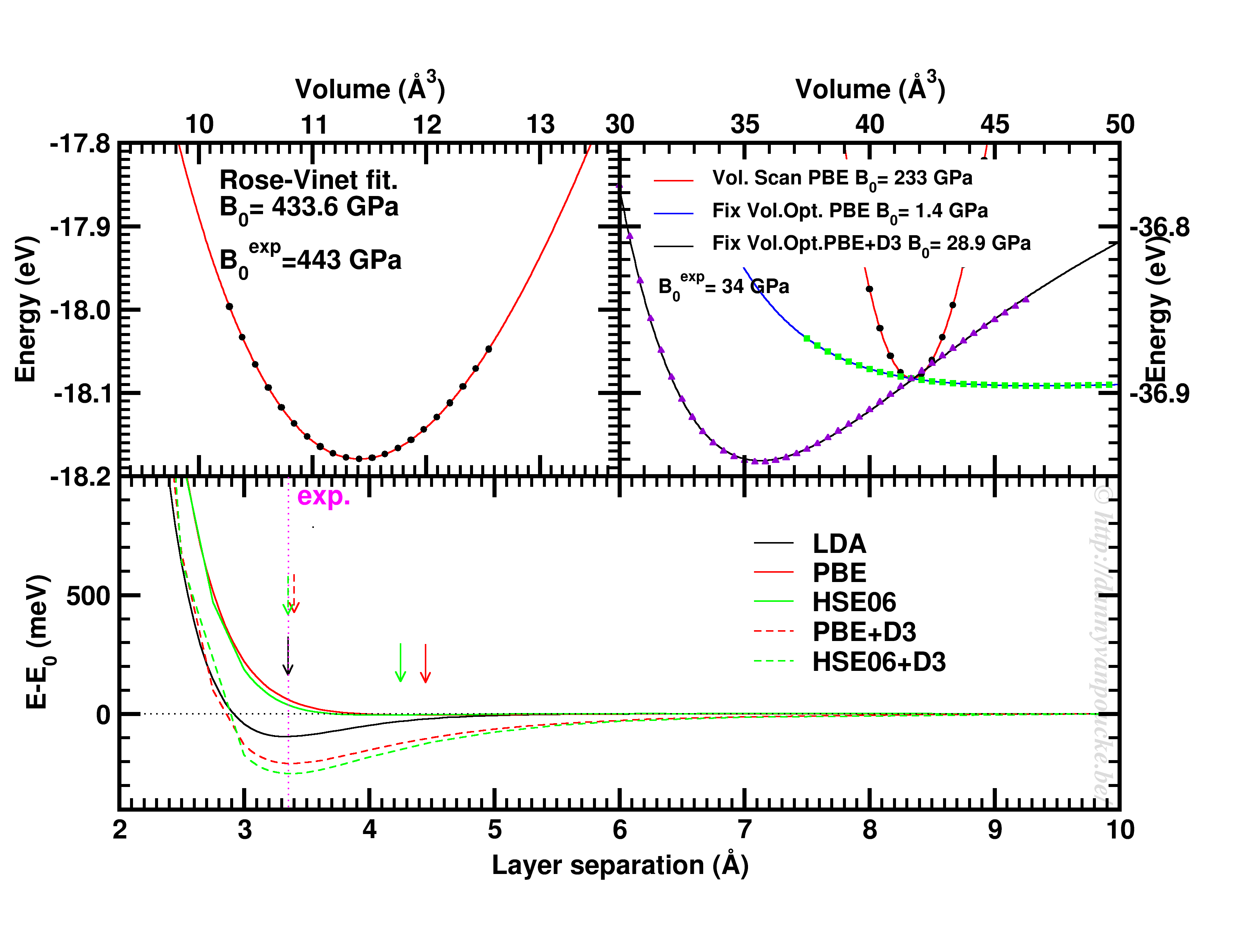
Top-left: Volume scan of Diamond. Top-right: comparison of volume scan and equation of state fitting to fixed volume optimizations, showing the role of van der Waals interactions. Bottom: Inter-layer binding in graphite for different functionals.
Let us start with a simple and well behaved system: Diamond. This material has a very simple internal structure. As a result, the internal coordinates should not be expected to change with reasonable volume variations. As such, a simple volume scan (option 3), will allow for a good estimate of the equilibrium volume. The obtained bulk modulus is off by about 2% which is very good.
Switching to graphite, makes things a lot more interesting. A simple volume scan gives an equilibrium volume which is a serious overestimation of the experimental volume (which is about 35 Å3), mainly due to the overestimation of the c-axis. The bulk modulus is calculated to be 233 GPa a factor 7 too large. Allowing the structure to relax at fixed volume changes the picture dramatically. The bulk modulus drops by 2 orders of magnitude (now it is about 24x too small) and the equilibrium volume becomes even larger. We are facing a serious problem for this system. The origin lies in the van der Waals interactions. These weak forces are not included in standard DFT, as a result, the distance between the graphene sheets in graphite is gravely overestimated. Luckily several schemes exist to include these van der Waals forces, the Grimme D3 corrections are one of them. Including these the correct behavior of graphite can be predicted using an equation of state fit to fixed volume optimizations.(Note that the energy curve was shifted upward to make the data-point at 41 Å3 coincide with that of the other calculations.) In this case the equilibrium volume is correctly estimated to be about 35 Å3 and the bulk modulus is 28.9 GPa, a mere 15% off from the experimental one, which is near perfect compared to the standard DFT values we had before.
In case of graphite, the simple volume scan approach can also be used for something else. As this approach is well suited to check the behaviour of 1 single internal parameter, we use it to investigate the inter-layer interaction. Keeping the a and b lattice vectors fixed, the c-lattice vector is scanned. Interestingly the LDA functional, which is known to overbind, finds the experimental lattice spacing, while both PBE and HSE06 overestimate it significantly. Introducing D3 corrections for these functionals fixes the problem, and give a stronger binding than LDA.
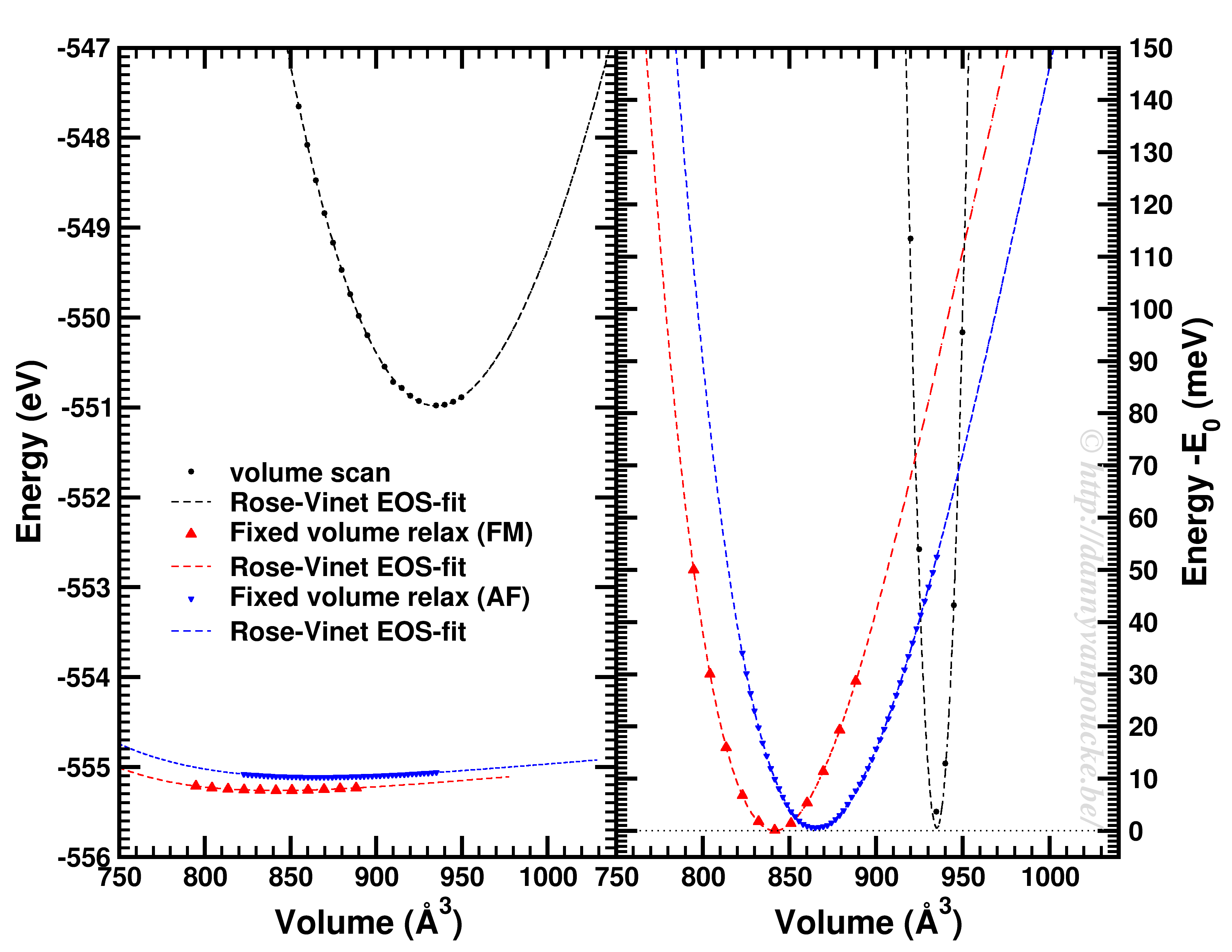
Comparison of a volume scan and an EOS-fit to fixed volume optimizations for a Metal-Organic Framework with MIL53/47 topology.
We just saw that for simple systems, the simple volume scan can already be too simple. For more complex systems like MOFs, similar problems can be seen. The simple volume scan, as for graphite gives a too sharp potential (with a very large bulk modulus). In addition, internal reordering of the atoms gives rise to very large changes in the energy, and the equilibrium volume can move quite a lot. It even depends on the spin-configuration.
In conclusion: the safest way to get a good equilibrium volume is unfortunately also the most expensive way. By means of an equation of state fit to a set of fixed volume structure optimizations the ground state (experimental) equilibrium volume can be found. As a bonus, the bulk modulus is obtained as well.
Permanent link to this article: https://dannyvanpoucke.be/vasp-tutor-eosfit-en/
Jan 01 2017
2016 has come and gone. 2017 eagerly awaits getting acquainted. But first we look back one last time, trying to turn this into a tradition. What have I done during the last year of some academic merit.
Publications: +4
Completed refereeing tasks: +5
Conferences: +4 (Attended) & + 1 (Organized)
PhD-students: +2
Current size of HIVE:
Hive-STM program:
Permanent link to this article: https://dannyvanpoucke.be/review-of-2016-en/
Dec 26 2016
When running programs on HPC infrastructure, one of the first questions to ask yourself is: “How well does this program scale?“
In applications for HPC resources, this question plays a central role, often with the additional remark: “But for your specific system!“. For some software packages this is an important remark, for other packages this remark has little relevance, as the package performs similarly for all input (or for given classes of input). The VASP package is one of the latter. For my current resource application at the Flemish TIER-1 I set out to do a more extensive scaling test of the VASP package. This is for 2 reasons. The first being the fact that I will be using a newer version of VASP: vasp 5.4.1 (I am currently using my own multiply patched version 5.3.3.). The second being the fact that I will be using a brand new TIER-1 machine (second Flemish TIER-1, as our beloved muk retired the end of 2016).
Why should I put in the effort to get access to resources on such a TIER-1 supercomputer? Because such machines are the life blood of the computational materials scientist. They are their sidekick in the quest for understanding of materials. Over the past 4 years, I was granted (and used) 20900 node-days of calculation time (i.e. over 8 Million hours of CPU time, or 916 years of calculation time) on the first TIER-1 machine.
Now back to the topic. How well does VASP 5.4.1 behave? That depends on the system at hand, and how good you choose the parallelization settings.
VASP provides several parameters which allow for straightforward parallelization of the simulation:
In addition, one needs to keep the architecture of the HPC-system in mind as well: NPAR, KPAR and their product should be divisors of the number of nodes (and cores) used.
Both NPAR and KPAR parameters can be set simultaneously and will have a serious influence on the speed of your calculations. However, not all possible combinations give the same speedup. Even worse, not all combinations are beneficial with regard to speed. This is best seen for a small 2 atom diamond primitive cell.
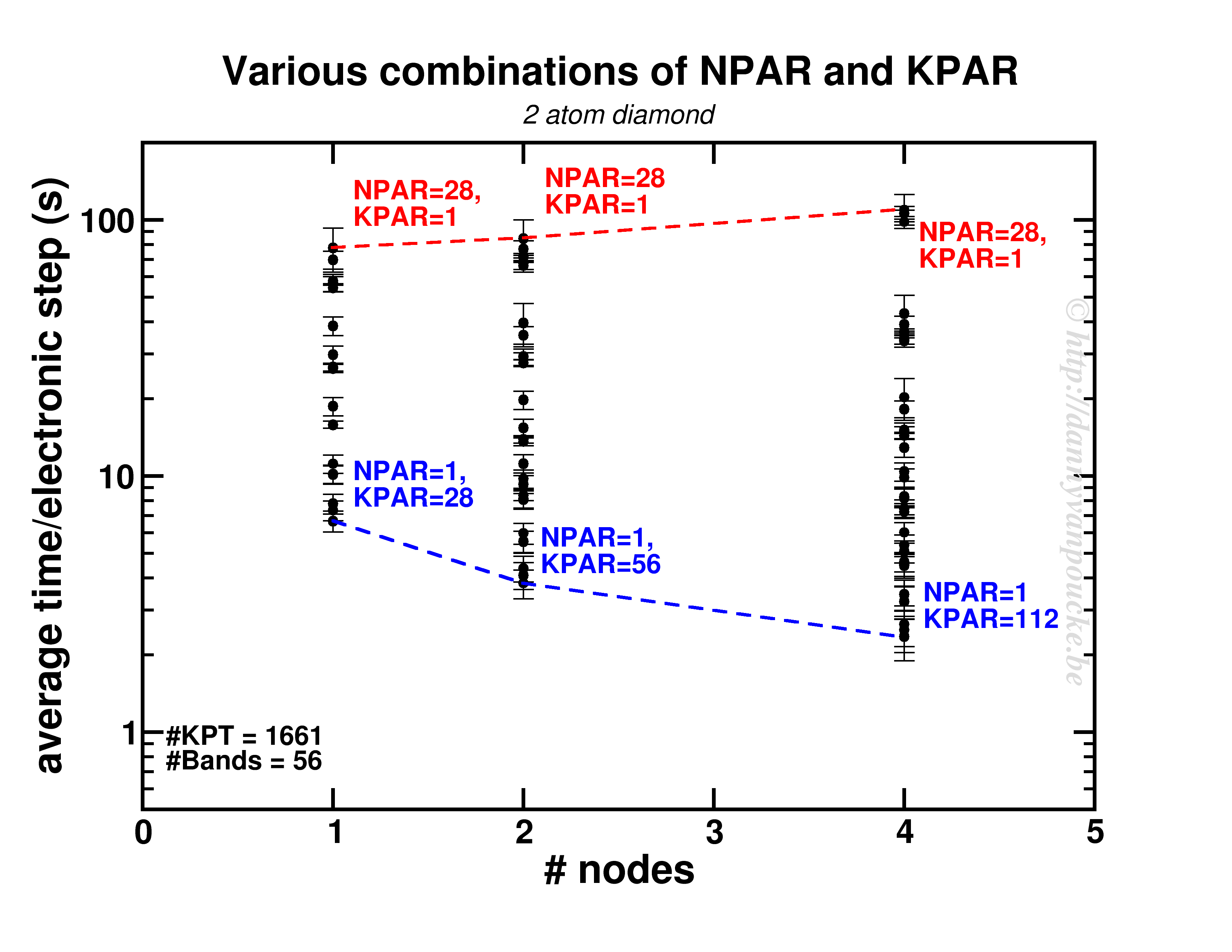
Timing results for various combinations of the NPAR and KPAR parameters for a 2 atom primitive unit cell of diamond.
Two things are clear. First of all, switching on a parallelization parameter does not necessarily mean the calculation will speed up. In some case it may actually slow you down. Secondly, the best and worst performance is consistently obtained using the same settings. Best: KPAR = maximal, and NPAR = 1, worst: KPAR = 1 and NPAR = maximal.
This small system shows us what you can expect for systems with a lot of k-points and very few electronic bands ( actually, any real calculation on this system would only require 8 electronic bands, not 56 as was used here to be able to asses the performance of the NPAR parameter.)
In a medium sized system (20-100 atoms), the situation will be different. There, the number of k-points will be small (5-50) while the natural number of electronic bands will be large (>100). As a test-case I looked at my favorite Metal-Organic Framework: MIL-47(V).
Timing results for several NPAR/KPAR combinations for the MIL-47(V) system.
This system has only 12 k-points to parallelize over, and 224 electronic bands. The spread per number of nodes is more limited than for the small system. In contrast, the general trend remains the same: KPAR=high, NPAR=low, with an optimum performance when KPAR=#nodes. Going beyond standard DFT, using hybrid functionals, also retains the same picture, although in some cases about 10% performance can be gained when using one half node per k-point. Unfortunatly, as we have very few k-points to start from, this will only be an advantage if the limiting factor is the number of nodes available.
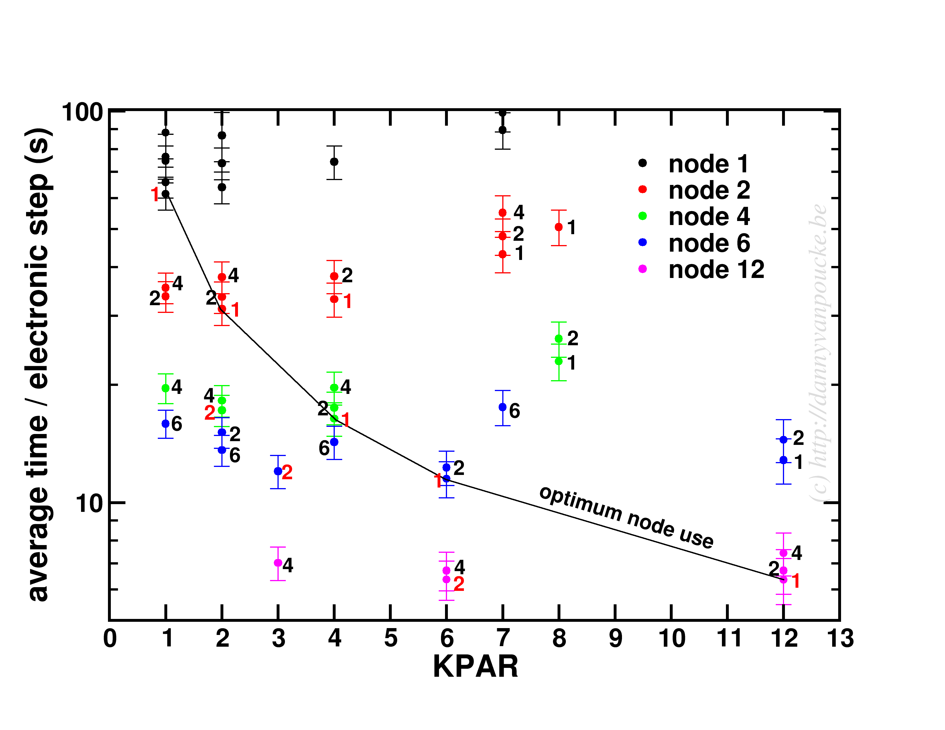
An interesting behaviour is seen when one keeps the k-points/#nodes ratio constant:
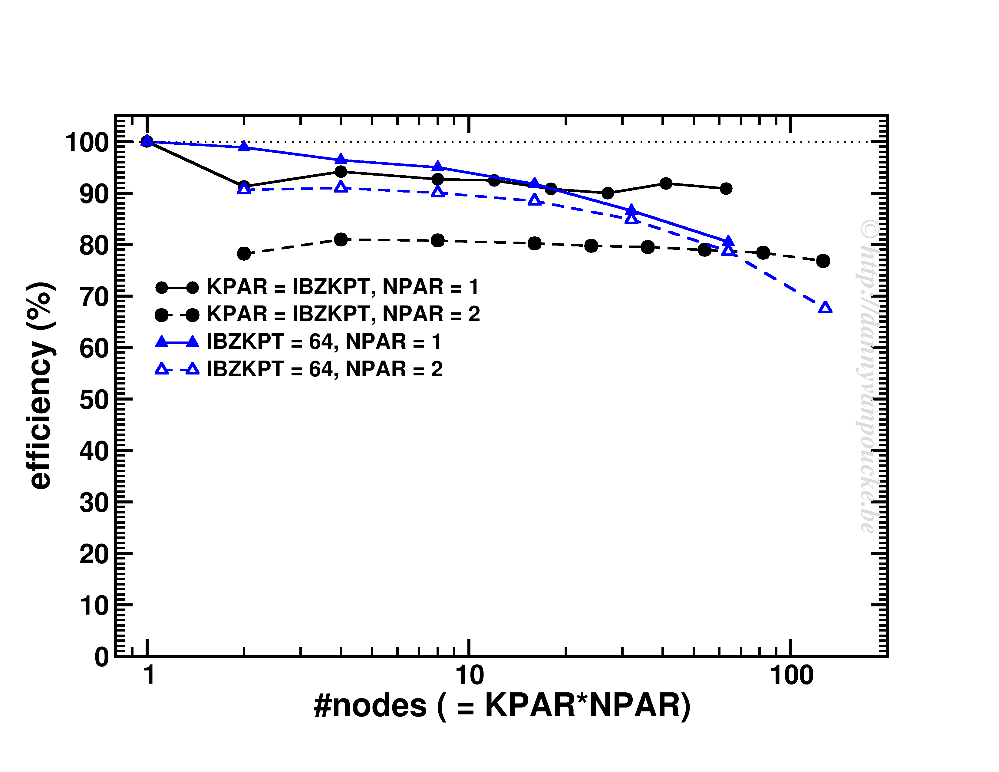
Scaling behavior for either a constant number of k-points (for dense k-point grid in medium sized system) or constant k-point/#nodes ratio.
As you can see, VASP performs really well up to KPAR=#k-points (>80% efficiency). More interestingly, if the k-point/#node ratio is kept constant, the efficiency (now calculated as T1/(T2*NPAR) with T1 timing for a single node, and T2 for multiple nodes) is roughly constant. I.e. if you know the walltime for a 2-k-point/2-nodes job, you can use/expect the same for the same system but now considering 20-k-points/20-nodes (think Density of States and Band-structure calculations, or just change of #k-points due to symmetry reduction or change in k-point grid.) 😆
If one thing is clear from the current set of tests, it is the fact that good scaling is possible. How it is attained, however, depends greatly on the system at hand. More importantly, making a poor choice of parallelization settings can be very detrimental to the obtained speed-up and efficiency. Unfortunately when performing calculations on an HPC system, one has externally imposed limitations to work with:
Here are some guidelines (some open doors as well):
In short:
[1] 28 is a lousy number in that regard as its prime-decomposition is 2x2x7, leaving little overlap with prime-decompositions of the number of k-points, which more often than you wish end up being prime numbers themselves 😥
[2] The small system’s memory requirements varied from 0.15 to 1.09 Gb/core for the different combinations.
Permanent link to this article: https://dannyvanpoucke.be/scaling-vasp-breniac-en/